Some of the above gene classes are deduced from the gene name supplied
with the Gene In Plate Order (GIPO) file for the array. We use the
following automatic classification rules shown in Table 2.4.1.
 Filter by current Ordered
Condition List (OCL) F-Test [p-Value] slider [RB] - only
include genes that meet the F-test criteria on the current
OCL. This only works if there are at least 2 (replicate)
samples/condition for each of the condition sets in the OCL.
See info on defining
the OCL and
using the OCL data.
Filtering out genes with high replicate spot variation
The Spot CV filter mode submenu contains options to select how
the spot CV filter is to be applied. It computes the maximum value of
CV for all of the samples in the particular sample set specified. That
maximum value is then used for the spot CV filter test. Genes may be
filtered out having a large difference between spot quantification
values of corresponding duplicate spots. You may compute the
coefficient of variation CVj for the two values
(f1j and f2j for a particular
gene j.
CVj = 2|f1j-f2j|/(f1j+f2j)
If the database only has one field but replicate HPs, then you may use
the HP-X & HP-Y 'sets' CVj to filter the
genes. Then CVj values are tested against a CV
threshold slider value to eliminate genes with a high coefficient of
variation.
-
 Current HP [RB] - CV of (F1,F2) for each gene in current
sample [if duplicate spots are available on each sample]
-
 HP-X or HP-Y [RB] -
CV of (F1,F2) for HP-X and HP-Y single samples [if duplicate
spots are available on each sample]
-
 HP-X 'set' [RB] - CV of spots in HP-X set
-
 HP-Y 'set' [RB] - CV of spots in HP-Y set
-
 HP-X or HP-Y 'sets' [RB] - CV of spots in the HP-X set or HP-Y
set
-
 HP-X and HP-Y 'sets' [RB] - CV of spots in both the HP-X
set and HP-Y set
-
 HP-E [RB] - CV of HPs in expression profile list
Any or all of the data filters may be selected simultaneously. In
particular, if you select filters that use parameter threshold
scrollers, they will be added to a state scroller window (see Figure
2.3.4.1 for details to allow adjustment of ALL sliders
simultaneously). You may change various thresholds and see the effect
in real time. Note: some of the scrollers are more sensitive to low
values. Therefore, we set them to respond non-linearly with a more
precise vernier at the low end.
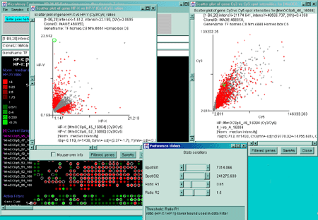
Figure 2.4.3.1 Filtering using multiple scrollers. This example
is of Cy3/Cy5 time series data. It filters normalized spot intensity
of the Cy3 and Cy5 channels independently ([SI1:SI2] inside range)
where low intensity spots are eliminated. It then filters out genes
outside of the [R1:R2] ratio range.
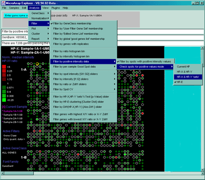
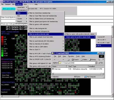
Figure 2.4.3.2 Using the Positive Intensity data Filter.
This allows removing negative data if the data contains negative
intensity values (e.g. Some Affymetrix data has negative Average Difference
values which could be read as Intensity for MAExplorer).

MAExplorer - Microarray Exploratory Data Analysis
The Plot menu lets you display a pseudoarray image, scatter plots,
ratio and intensity histograms,and expression profile plots. The
pseudoarray image is displayed in the main MAExplorer window. All of
the other plots are displayed in popup windows. Depending on the
particular plot, multiple instances may be allowed. The Plot
submenus are:
- Show Microarray
 - display the pseudoarray image
for the current HP sample
- Scatter plots
 - display various scatter plots
of selected pairs of HP samples
- Histograms
 - display both ratio and
intensity histograms of HP sample data
- Expression profile plots
 - display expression profile
plots of genes or gene subsets
You may switch between different representations of the microarray
spot pseudoarray image. It may be viewed as several different types of
pseudo images including an intensity gray value and a pseudo-color
Red/Black/Green image for ratio (HP-X/HP-Y) and Zscore (HP-X - HP-Y)
data. The p-Value results of comparing a HP-X 'set' with a HP-Y 'set'
of samples, or the CV of the HP-EP 'list can be displayed as a color
spectrum pseudoarray image.
Depending on the origin of the array data, it may have the same
verisimilitude as the original arrays. Otherwise, it is displayed in
a generic pseudoarray image containing grids that will fit the window
- these are not the same as the original array image (see . However, the
pseudoarrays are useful to getting a rough idea of the global changes
in the data between arrays and how may genes pass the data filter.
When enabled using one of the commands in the Section 2.4.5 Clustering menu, cluster data appears as
blue circles or squares drawn as overlays on
the pseudoarray image. These options are discussed in the section on
clustering. If you are doing clustering K-means clustering, the
current cluster is displayed in the scatter plot if the latter is
active.
Scatter plots, ratio and intensity histograms of the mean (HP-X/HP-Y)
or (HP-X/HP-Y) 'set' data, or the F1/F2 or Cy3/Cy5 data. F1/F2
or Cy3/Cy5 plots are available if the data exists in your particular
database. That might be the case with replicate spots or with Cy3/Cy5
data. If the normalization is set to a Zscore or log mean mode, it
will compute Zscore scatter plots and histograms.
Clicking on spots in an array image or points in scatter plots sets
the current gene and will bring up data on the gene or (optionally)
access corresponding data from GenBank, UniGene, mAdb Clone, etc. databases in a
popup Web browser. Clicking on a bin in a ratio or intensity
histogram plot filters out all genes except for those in the range of
that bin.
Expression profiles plots of selected genes or subsets of genes for
all samples in the HP-E list. These are active plots with data reported
when the user clicks in the plot.
Clicking on a spot (i.e. gene) in the microarray pseudo image or on a
point (i.e. gene) in the scatter plot, it will define that gene as the
"current gene" that is used in other operations. The current gene is
indicated in both plots with a green circle
around it. Similarly, you may modify
the 'Edited Gene List' from either the pseudoarray image or the
scatter plot. When viewing is enabled, it overlays those genes with
magenta squares.
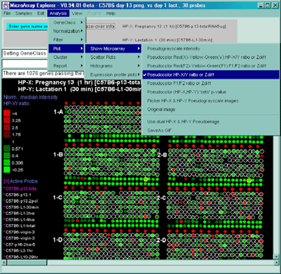
Figure 2.4.4 Plot menu - selecting Ratio Pseudoarray
image. This displays a pseudocolor show in the scale on the left that
indicates the ratio of the value of the HP-X sample / HP-Y sample (or
'sets' if the option to use HP-X and HP-Y 'sets' is enabled.) If The
data is Cy3/Cy5 data, then this displays the ratio of the ratios using
the current normalization. Various other pseudoarray image
representations could be used.
You may show the pseudoarray
image of the current hybridized samples using several
modalities. The grayscale pseudoarray image is generated from the
quantified spot data. If the data contains the actual spot positions
of the genes (as generated by the various array image quantification
program), the spots may be drawn using a scaled version of those
coordinates. Otherwise, a generic set of grids (and fields in there
are multiple fields) is synthesized to represent the spot
positions. Pseudoarray images may also be useful as an alternative
modality for displaying X/Y ratio or X-Y Zdiff data. If the
normalized intensities are the same, then the spot will appear as
black with the overall spot intensity depending on the spot
concentrations. High ratios and Zdiffs will be red and low values
green as shown in Table
2.4.4.1. The p-Value results of comparing a HP-X 'set' with a
HP-Y 'set' of samples can be displayed as a color spectrum pseudoarray
image.
If the database that was loaded contains only one sample, the
pseudoarray image display defaults to the pseudograyscale spot
intensity mode. If there is at least one HP-X and one HP-Y sample,
then the Pseudocolor HP-X/Y ratio or Zdiff mode is the initial
default display. If there are duplicate spots for each gene, you may
generate a Pseudocolor F1F2 ratio or Zdiff mode image. If you
are using Cy3/Cy5 ratio data and the data is available as independent
channels for each HP, then you may plot Cy3 vs Cy5 for individual
samples.
When available on the database server, the original image may be
displayed in a separate popup Web browser.
Table 2.4.4.1. Pseudocolors assigned to spots to represent data in
the X/Y ratios or X-Y Zdiffs pseudocolor array images. Each color
represents the normalized X/Y ratio or X-Y Zdiff depending on
Normalization mode. The 9 colors of the boxes represent the normalized
expression ranges.
| . |
. |
. |
. |
. |
. |
. |
. |
. |
Normalization
mode - RBG |
| bright green |
. |
. |
dark green |
Black |
dark red |
. |
. |
bright red |
| . |
. |
. |
. |
. |
. |
. |
. |
. |
Normalization
mode - dichromasy |
| bright blue |
. |
. |
dark blue |
Black |
dark orange |
. |
. |
bright orange |
| <0.250X |
0.307X |
0.400X |
0.571X |
1.000X |
1.75X |
2.50X |
3.25X |
>4.00X |
Ratio data |
| <-3.0 |
-2.25 |
-1.50 |
-0.75 |
0.00 |
0.75 |
1.50 |
2.75 |
>3.0 |
Zscore data |
| <-0.99 |
-0.742 |
-0.495 |
-0.247 |
0.000 |
0.247 |
0.495 |
0.742 |
>0.99 |
Zscore Log data |
Clicking on a particular gene will report its specific quantification
and identification values (See
Section 3.3 on gene quantification). If the Enable display current
gene in popup genomic DB Web Browser option is set in the
View menu, then it will also pop up a Web browser with the
corresponding to the particular genomic DB data for that
database if it exists.
The same data is shown in a variety of normalization and display formats.
The relative intensity may be displayed for the current sample (last
HP-X or HP-Y selected) or two samples (HP-X or HP-Y samples or HP-X or
HP-Y 'sets' of samples). To show two samples side by side, enable the
Use dual HP-X & HP-Y Pseudoimage in the Show Microarray
submenu. To show averaged set data in the dual mode, enable the "Use
HP-X & HP-Y 'sets' option in the Samples menu. The grayscale
value reflects the current normalization mode.

Figure 2.4.4.1.1.1 Pseudoarray intensity image of median normalized
intensities of the current HP sample (C57B6 virgin 10 weeks from MGAP
database). The graylevel scale on the left edge of the pseudoarray
image indicates the spot intensity. All pseudoarray images have scales
that vary depending on the type of pseudoarray being displayed.
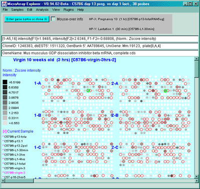
Figure 2.4.4.1.1.2 Pseudoarray intensity image of Zscore normalized
intensities of the current HP (C57B6 virgin 10 weeks from MGAP
database).
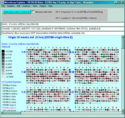
Figure 2.4.4.1.1.3 Pseudoarray intensity image of ZscoreLog normalized
intensities of the current HP (C57B6 virgin 10 weeks from MGAP database).

Figure 2.4.4.1.1.4 Pseudoarray intensity image of ZscoreLog
normalized intensities of the dual HP-X and HY-Y individual
samples. The Plot menu Show Microarray submenu toggle "Use dual
HP-X & HP-Y samples" option is set. HP-X is a C57B6 pregnancy day
13 and HP-Y is a Stat5a (-,-) pregnancy day 13.
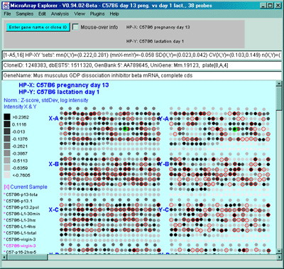
Figure 2.4.4.1.1.5 Pseudoarray intensity image of ZscoreLog
normalized intensities of the dual HP-X and HY-Y sample 'sets'. The
Plot menu Show Microarray submenu toggle "Use dual HP-X & HP-Y
samples" option is set. The "Use HP-X & HP-Y 'sets' option in the
Samples menu. HP-X is the mean of three 'C57B6 pregnancy day 13' and
HP-Y is the mean of three 'Stat5a (-,-) pregnancy day 13'.
The ratio (HP-X/HP-Y) or Zdiff HP-X - HP-Y) normalized intensity data
may be displayed as a pseudoarray image for HP-X and HP-Y, or HP-X and
HP-Y 'sets' of samples. To show averaged set data in the dual mode,
enable the "Use HP-X & HP-Y 'sets' option in the Samples menu.
The colors of the 9 scale boxes represent the normalized expression
ranges and is assigned according to the current normalization mode
listed in the table.

Figure 2.4.4.1.2.1 Pseudocolor array image of median normalized X/Y
ratios. HP-X is C57B6 pregnancy day 13 and HP-Y is Stat5a (-,-)
pregnancy day 13. Each spot's color represents the normalized X/Y
ratio depending on Normalization mode. The color of the box is one of
9 colors representing the normalized expression ranges and assigned
according to the table "Ratio
mode".
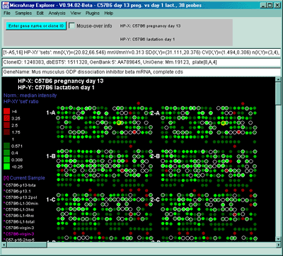
Figure 2.4.4.1.2.2 Pseudoarray color image of normalized X/Y 'set'
mean value ratios. Mean of three HP-X C57B5 pregnancy day 13
samples and mean of three HP-Y Stat5a (-,-) pregnancy day 13 samples.
Each spot's color represents the normalized X/Y 'set' ratios depending
on Normalization mode. The color of the box is one of 9 colors
representing the normalized expression ranges and assigned according
to the table "Ratio mode".
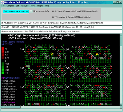
Figure 2.4.4.1.2.3 Pseudoarray color image of X-Y Zdiffs. HP-X
is C57B6 pregnancy day 13 and HP-Y is Stat5a (-,-) pregnancy day 13.
Each spot's color represents the normalized X-Y Zdiff depending using
the Zdiff normalization mode. The color of the box is one of 9 colors
representing the normalized expression ranges and assigned according
to the table "Zdiff mode".

Figure 2.4.4.1.2.4 Pseudoarray color image of X-Y Zdiff of log
data. HP-X C57B5 pregnancy day 13 sample and HP-Y Stat5a (-,-)
pregnancy day 13 sample. Each spot's color represents the normalized
X/Y ratio depending on ZdiffLog with StdDev normalization mode. The
color of the box is one of 9 colors representing the normalized
expression ranges and assigned according to the table "ZdiffLog mode".
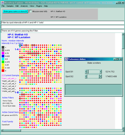
Figure 2.4.4.1.2.5 Pseudoarray image showing color-coded p-values
for t-test comparison of HP-X and HP-Y 'set' samples. The HP-X and
HP-Y sets both have 2 samples each (more is obviously much better).
The data was normalized using the Median and a spot intensity
[SI1:SI2] data filter was applied to eliminate some of the noisy data.
Each spot's color represents a p-value in the range indicated in the
scale in the left edge of the image. Note that although all spots are
assigned a p-Value, many may not be very significant because adequate
preprocessing of the data (such as normalization, and low intensity
spot removal, etc.). So use this display with care.
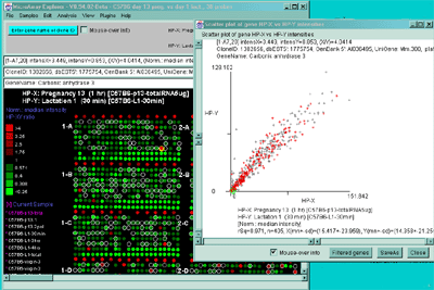
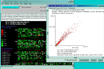
Scatter plots include HP-X vs HP-Y intensity for comparing data
between HP-X and HP-Y samples (or sets if the HP-X and -Y sample
'sets' mode is enabled in the Samples menu - as is shown in Figure 2.2.1). You may
zoom into any area of the scatter plot as is shown in Figure
2.4.4.4.2(C). If there are duplicate spots for each gene, you may
plot F1 vs F2 intensity (or Cy3 vs Cy5 if using ratio data) for
comparing replicate data (or Cy3 and Cy5 ratio data channels) within
the same sample It will also compute the correlation coefficient for
the data and display it in the plot and in the message panel. The data
is the intensity values using the current normalization method. If you
are analyzing ratio Cy3/Cy5 data, you may compare Cy3 or Cy5 of the
HP-X sample against Cy3 or Cy5 of the HP-Y sample. If you are in
stand-alone mode, a SaveAs GIF button will also be
available. This saves the current plot as a full resolution GIF file
specified by the user in a popup file browser window.
rSq=0.974, n=1728, X(mn+-sd)=(4.477+-7.845), Y(mn+-sd)=(12.379+-24.810)
The Scatter plots submenu includes:
- HP-X vs HP-Y intensity - display a scatter plot of HP-X
vs HP-Y intensity data of H.P. selected (average of F1+F2
fields). If HP-X/-Y 'sets' are enabled, then the plot is of the
mean set values.
- HP F1 vs F2 intensity - display a scatter plot of F1 vs F2
(or Cy3 vs Cy5) intensity data of the current selected sample
- --------------------
- HP-X Cy3 vs HP-Y Cy3 intensity - display a scatter plot of
HP-X(Cy3) vs HP-Y(Cy3) intensity data of the currently selected
HP-X and HP-Y samples (ratio data only).
- HP-X Cy5 vs HP-Y Cy5 intensity - display a scatter plot of
HP-X(Cy5) vs HP-Y(Cy5) intensity data of the currently selected
HP-X and HP-Y samples (ratio data only).
- HP-X Cy3 vs HP-Y Cy5 intensity - display a scatter plot of
HP-X(Cy3) vs HP-Y(Cy5) intensity data of the currently selected
HP-X and HP-Y samples (ratio data only).
- HP-X Cy5 vs HP-Y Cy3 intensity - display a scatter plot of
HP-X(Cy5) vs HP-Y(Cy3) intensity data of the currently selected
HP-X and HP-Y samples (ratio data only).
If Cy3/Cy5 ratio data is being analyzed, then the "HP F1 vs F2
intensity" menu entry becomes
- HP Cy3 vs Cy5 intensity - display a scatter plot of Cy3 vs
Cy5 intensity data of the current sample selected (i.e. being
displayed).
The following figure illustrates some of the scatter plots and zoomed
regions using the scroll bars on the horizontal and vertical axes.
A)
B)
C)

Figure 2.4.4.2 Scatter plot of HP-X and HP-Y single sample
data. HP-X is C57B6 pregnancy day 13 and HP-Y is pactation day 1.
A) An active scatter plot may be generated for the current HP-X
and HP-Y samples filtered by "All named genes". B) similar
plot for HP-X and HP-Y 'sets' of replicate samples (3 pregnancy and 4
lactation samples in the sets respectively). Clicking on a point in
the plot sets the current gene. C) Zoomed up region (of
B) at the bottom of the plot showing more detail and filtered
by just "All named genes". Zooming is performed by adjusting the X or
Y axes limits scroll bars. Note the points enclosed in magenta boxes
indicate genes in the E.G.L. gene list.
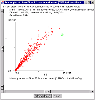
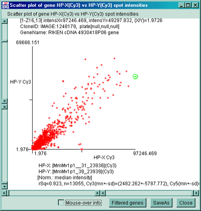
Scatter plots of data from multiple channels on the same sample
It is also possible to plot the separate channels within a single sample
against each other. For example F1 vs F2 in samples with replicate
data and Cy3 vs Cy5 in samples with separate ratio data channels.
A)
B)

C)
D)

Figure 2.4.4.2.1 Scatter plot of multiple channel data from a
single sample. A) F1 Vs F2 data for a C57B6 pregnancy day 13
sample. B) Cy3 vs Cy5 data for a NCI mAdb mouse array sample.
C) Scatter plot of individual Cy3 channels from two different
ratio Cy3/Cy5 data hybridized samples. C) Scatter plot of
individual Cy3 channel of HP-X compared with Cy3 channel of HP-Y for
ratio Cy3/Cy5 data hybridized samples. D) Scatter plot of
individual Cy3 channel of HP-X compared with Cy5 channel of HP-Y for
ratio Cy3/Cy5 data hybridized samples.
You may compare ratios or Zdiffs of data using the HP-XY ratios or
Zdiff command to display a ratio histogram of Filtered intensity
data from two samples selected from the Samples menu. The HP-XY
'set' ratio or Zdiff is used if there are multiple samples in the
HP-X or HP-Y sets, then the mean values in each of the sets is used in
the calculations. If there are duplicate spots for each gene, you may
plot the F1F2 ratio or Zdiff histogram of the F1/F2 ratios or
F1-F2 Zdiff values for normalized data for each spot in the currently
displayed sample. If you are in stand-alone mode, a SaveAs GIF
button will also be available to save the current plot as a full
resolution GIF file specified by the user in a popup file browser
window.
The Intensity selection plots a histogram of the gene intensity
data values for each Filtered spot (gene) in the current hybridized
sample.
The Histograms submenu includes:
- HP-XY ratio or Zdiff - display ratio or Zdiff histogram of data
from selected HP-X and HP-Y samples (mean F1+F2 data if duplicate
spots).
- HP-XY 'sets' ratio or Zdiff - display ratio or Zdiff histogram
of mean data from HP-X and HP-Y 'set's of samples (mean data).
- F1F2 ratio or Zdiff - display ratio or Zdiff of histogram of
F1 F2 duplicate spot data from the current sample.
- HP Intensity - (or HP (Cy3/Cy5) if ratio data) display a
histogram of spot intensity (or Cy3/Cy3 ratio) data for the current
sample.
If Cy3/Cy5 ratio data is being analyzed, then the F1F2 histogram menu
entry becomes
- Cy3Cy5 ratio or Zdiff - display ratio or Zdiff of histogram of
Cy3 Cy5data from the current sample.
The following figures illustrates the histograms. You may use the
histogram to specify ranges of [I1:I2] or {R1:R2] for data filtering
in the histogram by specifying the corresponding histogram bins. This
is described in the figure legend.
A)
B)
C)
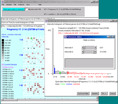
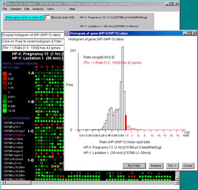
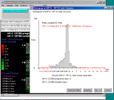
Figure 2.4.4.3 Histogram plots. A) Ratio histogram of
HP-X/HP-Y data with particular histogram bin selected with the
constraint set to filter all genes > that bin. HP-X is 13 day
pregnancy C57B6 and HP-Y is day 1 lactatation. The selected bin
thresholds are then used in the Filter with the resulting Filtered
genes shown in the array image. B) Zdiff histogram of HP-X -
HP-Y 'sets' for same data as (A) but with the ><
threshold constraint set to find genes outside of the symmetric
histogram range. C) Intensity histogram of HP-X data filtered
by [I1:I2] intensity range. As with ratio histograms, you can do
additional filtering by selecting a particular histogram bin that is
then used in the Filter. Filtering was disabled for the intensity
histogram. To apply the filter, the "Don't re-Filter" button would be
toggled to the "Re-Filter" state. The threshold constraints include:
=, >, <, >, <>, and ><. Note that each time
you click on the "Thr:" button, it cycles to the next option in the
threshold constraints list.
You may generate an individual expression profile plot (EP plot) or a
scrollable list of EP plots. The order list of hybridized samples to
plot are specified by the HP-E set. In the latter case, the genes are
specified by the data Filter.
You many generate as many individual expression profile plots as you
want using the Display a gene's expr. profile for HP-E
command. However, only the last one will be active and will be updated
with different genes as you click on them in the microarray image
scatter plot. This could be used to compare the EP plots for several
different genes. First view the EP plot for one gene, then create a
new EP plot for the second gene, etc.
If you use the Display Filtered genes expr. profiles
for HP-E command, it will generate a scrollable list of
expression profile plots for all of the genes passing the Filter. If
the number of genes is very large, it may take a while.
You may interrogate a line corresponding to a particular HP sample in
a EP plot by moving the mouse over the line and then selecting the
line. This will cause the name of the HP, its intensity and CV to
appear in the plot. If the Err check box is set, then the mean
of the intensity is indicated by a short horizontal bar and the +- CV
by red vertical error bars above and below the mean. If the plot
style Line button is pressed, then the plot style is cycled
between Line (vertical lines for each point), Circle (small circles at
each point), and Curve (circles are connected). Pressing the button
repeatedly cycles through: Line (i.e. vertical vars),
Circle, or Curve (i.e. continuous curve of all
samples). In the case of mean expression profiles
used in K-means clustering, the standard deviation is used in
place of the CV value. The various clustering methods have EP
plots buttons. When they are invoked, the scrollable list of EP
plots is sorted by the clustering method ordered list of genes. This
enables you to view the data in the same order as that produced by the
cluster analysis. If the zoom nnX button is pressed,
then all of the plots are magnified by nn-fold to make low intensity
plots more visible. Pressing the button repeatedly cycles through:
1X, 2X, 5X, 10X and 20X. It does not change the data itself. The
Show HP names button pops up a numbered list of all HP entries
used in the expression profile. If you are in stand-alone mode, a
SaveAs GIF button will also be available for the EP overlay
mode (Figure 2.4.4.4.1) or individual EP plot. This saves the current
plot as a full resolution GIF file specified by the user in a popup
file browser window.
The Expression profile plots submenu contains:
- Display a gene's expr. profile for HP-E - popup a window
and display the expression profile of a gene when click on a
spot in the Image or a point in the scatter plot.
- Display Filtered genes expr. profiles for HP-E -
popup a scrollable montage of expression profiles of the list
of Filtered genes.
- --------------------
 Use EP overlay else EP list [CB] - display Filtered genes
as an overlay plot of expression profiles, else as a scrollable
list of EP plots.
A)

B)
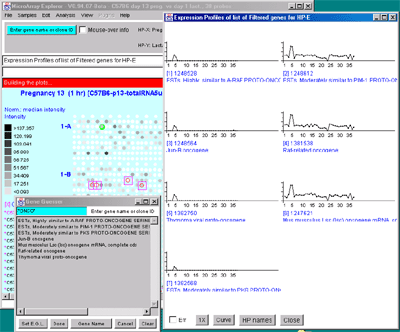
Figure 2.4.4.4 Expression profile plots. A) Individual
expression profile plots may be created by clicking on any
gene. Multiple instances may also be created. Here we show some of the
presentation options for the 38 sample MGAP database. Error bars are
computed for the standard error for that sample. There are three
different plotting options: line, circle and curve. #1 is the default
line plot with error bars. #2 is the line plot without the error bars
but clicking on line 7 to find out which sample it is and what the
intensity value is. #3 is the circle plot with error bars, and #4 is
the curve plot without error bars. Window #5 shows the list of samples
corresponding to the 38 points in the EP plots. B) List of
EPplots of the oncogenes and proto-oncogenes in the database (set by
the guesser with "onco" and "Set E.G.L." and the Edited Gene List
Filter). The list would become scrollable if there were more than 10
profiles. Setting the current gene would scroll the list to the EPplot
for the current gene.
A)
B)

C)
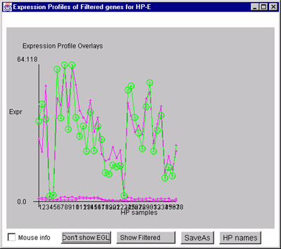
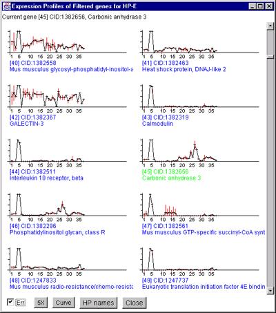
Figure 2.4.4.4.1 Expression profile plots.
A) Scrollable list of EP plots of Filtered named genes centered at
Carbonic anhydrase III.
B) Overlay plot of all named Filtered genes.
C) Overlay plot of all ONCO or PROTO-ONCO genes with the
draw EGL option active so the graphs are drawn for these genes.

MAExplorer - Microarray Exploratory Data Analysis
The Clustering menu lets perform various types of gene and condition
clustering operations. When you invoke a clustering operation it will
popup one or more windows and may modify the pseudoarray image. Some
of the popup windows include clustergram and dendrogram analysis plots
used with the hierarchical clustering.
When enabled, cluster data appears as blue circles
or squares drawn as overlays on the pseudoarray image. These
options are discussed in the section on clustering.
Cluster analysis plots include finding a subset of genes or subsets of
samples based on cluster analysis of expression profile similarity
measures. These show genes belonging to particular clusters, or genes
that cluster well with specified genes. Cluster methods include:
finding genes similar to the current selected gene within a "distance"
threshold; K-means-like clustering where you specify a seed gene and
the number of clusters; and hierarchical clustering with clustergram
and dendrogram graphics.
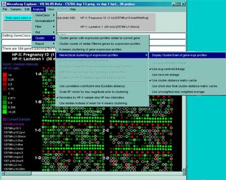
Figure 2.4.5 Cluster Menu options. The hierarchical clustering
option is being selected.
Use of clustering to find patterns of similar gene expression
Clustering is a way of possibly finding co-expressed genes that
exhibit similar expression changes in a set of samples. Genes may show
similar co-expression, but that does not prove they are co-regulated
at the same point in a pathway - merely that measurements of those
genes in a particular set of experiments show similar
expression. However, identifying genes with similar expression for
which some information is already known about some of the genes may be
useful as a starting point to help figure out gene function and
possibly aspects of its pathways in cell function using additional
experiments and analysis.
There are many methods for doing clustering - each with advantages and
disadvantages. We present three methods in MAExplorer and plan on
adding a variety of more powerful methods through the MAEPlugin
facility under development.
These methods may find genes belonging to particular clusters or genes
that cluster well with particular genes. Gene clusters are sets of
genes whose expression profiles are found to be similar according to a
particular metric. We now define what we mean by "similar". The order
list of hybridized samples used in computing the expression profiles
are those in the HP-E list. MAExplorer has two different dissimilarity
measures for Cij: Euclidean distance LSQdistij and Pearson correlation
coefficient rij. These are computed as
follows and are tested against the cluster distance threshold (set by
the slider in the preferences sliders). Let n= |HP-E|, the number of
samples in the expression profile. We define similarity as (1.0 -
normalized dissimilarity).
|
Hint: when working with very large data sets with many samples, it
may be useful to pre-adjust the distance and/or number of clusters
threshold sliders to an approximate range using the (Edit Menu |
Preferences | Adjust all Filter threshold scrollers). This is because
once the clustering starts, it does not (currently) let you abort the
clustering to change the threshold value.
|
   LSQdistij = Sqrt( Sum ( D'hj - D'hi) **2 ) / n
               h in HP-E
	       i,j in Filtered genes, i not j
Let,
   sumij = Sum( D'hj * D'hi ),
   mni = (1/n)Sum( D'hi ),
   mnj = (1/n)Sum( D'hj ),
   sumSqi = Sum( D'hi *  D'hi ),
   sumSqj = Sum( D'hj *  D'hj ),

then,
         [sumij - n*(mni * mnj)]
   rij = --------------------------------------------------------
         [Sqrt(sumSqi - n*n*mni*mni) * Sqrt(sumSqj - n*n*mnj*mnj)]
               h in HP-E
	       i,j in Filtered genes, i not j
The Cluster plots submenu contains a number of clustering
methods. Pressing the Escape key during a long cluster operation will
abort the operation. If you are in stand-alone mode using the
ClusterGram, a SaveAs GIF button will also be available for
saving the current plot as a full resolution GIF file specified by the
user in a popup file browser window.:
-
 Cluster genes with
expression profiles similar to current gene [RB] - click on
gene in image to find other genes with similar HP-E expression
profiles whose cluster distance is less than the cluster
distance threshold. The larger the blue
box, the higher the similarity.
-
 Cluster counts of
similar Filtered genes by expression profiles [RB] - draw
blue circles around filtered genes
indicating the number of other genes whose cluster similarity is
less than the cluster distance threshold. The larger the circle,
the more similar genes were found. Clicking on a gene switches
to the above mode.
-
 K-means clustering of
gene expression profiles [RB] - draw
magenta circles around the N primary-node gene clusters
representing the gene closest to representing the center of the
cluster. Each of the nodes is a maximum distance from all other
nodes in the recursive definition of nodes. N is determined by
the State Scroller "# of Clusters". Changing N will recompute
the clusters. It then pops up a scrollable text window with the
clusters and indicates which genes belong to it. If you select
the EP plot button, it will draw the expression profiles
for the clustered genes. The Mn-Cluster-Report button
will generate report for all genes sorted by K-means
cluster. Summaries can be generated using the Mean EP
plot and Mn-Cluster-Report buttons. The SaveAs
GeneSets button saves all of the clusters as named Gene Sets
("Cluster #1", "Cluster #2", etc). If you change the filter or
current gene, you should explicitly use the Recompute
Clusters button to regenerate the new set of clustered
genes. When you recompute the K-means clusters, it uses the
current gene as the initial node.
- Hierarchical clustering of expression profiles
 - this computes the hierarchical
clustering of the expression profiles (normalized by HP-X sample
data for each gene) of Filtered genes. The hierarchical
clusters are displayed in an ordered gene clustergram and
optional dendrogram. Sub-regions of the clustergram may be
explored in more detail using the EP-subset plot button,
or a report of the ordered genes can be created using the
ClustGram Report Note: you may add (remove) genes you
select from the Clustergram to the E.G.L. by holding the
Control(Shift) key while clicking on the gene name.
-
 S.O.M. gene clusters by
expr profiles [RB] - [Future MAEPlugin]
-
 Multi-Dimensional
Scaling of genes by expr profiles [RB] - [Future MAEPlugin]
-
 Multi-Dimensional
Scaling of genes by exprprofiles [RB] - [Future MAEPlugin]
-
 Clusters of (HP-E)
samples as fct of Filtered genes [RB] - [Future]
- --------------------
-
 Use correlation-coefficient
else Euclidian-distance [CB] - use the (1.0 - correlation
coefficient) as the distance metric instead of the default
Euclidean distance.
-
 Scale EP vector by max
magnitude prior to clustering [CB] - scale each sample in
the EP by the max magnitude for all sample values in the EP.
 Normalize by HP-X sample else
HP max intensities [CB] - normalize data by the
corresponding HP-X sample data for each gene or the maximum raw
intensity for each HP in the expression profile.
 Use median instead of mean
for K-means clustering [CB] - use the clustering (see (Bickel, 2001)).
The Hierarchical Cluster plots submenu contains:
-
 Display ClusterGram of gene
expr profiles [CB] - compute the hierarchical clustering of
the expression profiles (normalized by HP-X sample data for each
gene) of Filtered genes. Then display the hierarchical clusters
in an ordered gene clustergram and optional dendrogram when the
dendrogram checkbox is selected. Expression profile
plots of the clustergram may be explored in more detail using
the EP plot button that generates a scrollable list of
all EP plots ordered by the same order as the clustergram. A
full report of the ordered genes expression profiles may be
created using the ClustGram Report button.
- --------------------
-
 Use avg-arithmetic-linkage [RB] - set the hierarchical
clustering linkage method to the average arithmetic linkage of
sub-clusters.[ Future]
-
 Use avg-centroid-linkage
[RB] - set the hierarchical clustering linkage method to
average centroid linkage of sub-clusters (default).
-
 Use next-min-linkage
[RB] - set the hierarchical clustering linkage method to the
next minimum distance sub-cluster linkage in random order.
-
 Use cluster-distance matrix
cache [CB] - if you do not have enough memory for clustering
large gene sets, disable the cache. It will take MUCH longer
without the cache. When clustering, if there is
not enough memory available for the cache, it will warn you and
suggest you either reduce the number of genes being clustered or
use a computer with more memory.)
-
 Use short else float
cluster-distance matrix cache [CB] - if there is not enough
memory for the set of genes you wish to cluster and you still
want to use the cache, you can use 16-bit (i.e. short) data
instead of the 32-bit (i.e. float) data. The results will be
less precise.
-
 Use un-weighted else
weighted average [CB] - set the hierarchical clustering vector
averaging to un-weighted (the default weights it by the number
of genes in that sub-cluster). Otherwise using weighted gives
equal (0.50) weighting to each sub-cluster.
Handling of hierarchical clustering of large numbers of genes -
problem with slow response
The hierarchical clustering algorithm uses a gene-gene floating
point (i.e. 32-bit) distance matrix of order N2 (for N data
filtered genes). This means that if you are experiencing a slow
response, this may be due to several factors some of which you may not
be able to control. You might:
- If you determine that your computer is "paging", use a computer with
more memory. The currently distributed stand-alone version will use
up to 256 Mbytes of chip memory.
- If that is not possible, reduce the number of genes being clustered.
Even if you have enough memory, the computation is still high if N is
large.
- Set the Use short else float cluster-distance matrix cache
option in the cluster plot menu. This reduces the memory requirements
for the distance matrix by 1/2.
The Cluster genes with expression profiles similar to current
gene is used to find genes with similar HP-E expression profiles
as measured by the least square error that are less than the cluster
distance threshold. It pops up the "Cluster Distance" threshold
scroller. Then click on a gene in the microarray image. It then pops
up up a window with a list of the similar genes and their expression
profile distances to the current gene. Each gene that passes the
cluster distance threshold test is indicated in the image with a blue square where the size of the square is
proportional to its similarity. It also displays a sorted list of the
genes with the cluster distance in the cluster panel that was popped
up. On each lines is a series of '*****' - the more stars the higher
the similarity to the seed gene. This is a silhouette plot that
is used to display a sorted list of similar objects and is described
to that described in (Kaufman and
Rousseeuw, 1990).
Larger squares indicate that more genes are similar. You may
change the cluster distance threshold and it will update the display
and the list. In addition, the 'edited gene list' is set to the
subset of genes that belong to the current cluster.
A)
B)
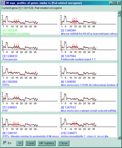
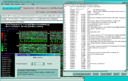
Figure 2.4.5.1 Similar genes clustered to the current gene.
This method finds all genes that are similar to the current gene as
those defined by their distance between expression profiles being less
than the threshold set by the user. Each gene that passes the cluster
distance threshold test is indicated in the image with a blue square where the size of the square is
proportional to its similarity. This data is from the 38 samples in
the MGAP database containing duplicated spots. A) Main windows
with popup cluster similarity report and cluster distance threshold
slider. B) Scrollable list of EPplots of similar genes with the
red error bars indicating the variation for duplicated spots for each
HP sample. The Err checkbox may turn the error bar overlays on
and off.
The Cluster counts of similar Filtered genes by expression
profiles command analyzes the set of all Filtered genes for the
expression profile defined by the HP-E samples. It counts the number
of similar genes for each Filtered gene and draws a
blue circle whose size is proportional to the number of genes
similar to that gene. After it analyses these genes it lists the
genes and their counts in the cluster panel. You may change the
cluster distance threshold and/or Filter parameters and it will update
the display and the list. If you click on a gene with a green circle, it will switch to single gene
cluster mode (with the blue squares).
For both of these commands, if you want to view the expression profile
plots, click on the EP plot button in the cluster window and it
pops up the scrollable expression profiles window. If you click on a
gene in the image, it will select it as the new current gene and seed
gene and recompute the cluster of genes most similar to the new see
gene.
For both of these commands, if you want a permanent report, click on
the "Cluster Report" button in the cluster window and it will generate
a report in the current modality (i.e. scrollable spreadsheet or
tab-delimited). You may switch between these two modes by pressing
the "Go '...'" button in the report.
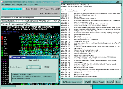
Figure 2.4.5.2 Display of cluster counts for all genes less than
the cluster threshold from MGAP 38 sample database. The algorithm
counts the number of similar genes for each Filtered gene and draws
a blue circle whose size is proportional to
the number of genes similar to that gene. That is why there are a larger
number of the larger circles.
The K-means cluster gene expression profiles for Filtered genes
command searches the data Filtered gene list for the genes
(i.e. primary genes) with the N most orthogonal expression
profiles. It will start this recursive computation from the gene with
minimum distance to all other genes unless you have selected a
"current gene" with the mouse. All Filtered genes are assigned to the
nearest K-means primary node. The mean cluster vector is computed and
used as the new definition of the cluster center. If you set the "Use
median instead of mean for K-means clustering" option in the
Clustering submenu, it will compute the center as a median instead of
a mean (Bickel, 2001). K-means
clustering is described in (Sneath
and Sokol, 1973). A new K-means primary gene (i.e. gene for the
cluster center) is found that is closest to this new center. Then all
of the data Filtered genes are reassigned to the new cluster
centers. The mean+-stdDev of the within-cluster distance to its center
is computed. It then pops up a text window with an ordered report of
the Filtered genes illustrated by part of a report shown below. [This
is part of a report from a 38 sample MGAP database subset of 141 genes
from the set of named genes restricted by the CV data filter.] Note
that clusters where the "Similarity" data is plotted as a silhouette plot use
variable length strings of '****' is about the same for the entire
cluster (e.g. cluster #4) contain genes that probably belong together
in the same cluster. Clusters that do not (e.g. Cluster 6) probably
contain two smaller more robust clusters.
A)
B)
C)
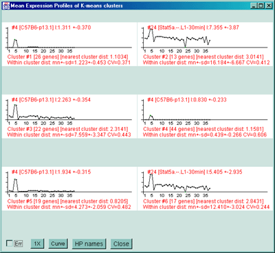
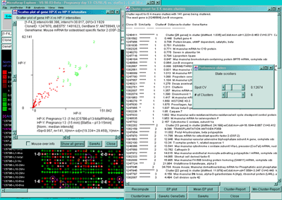
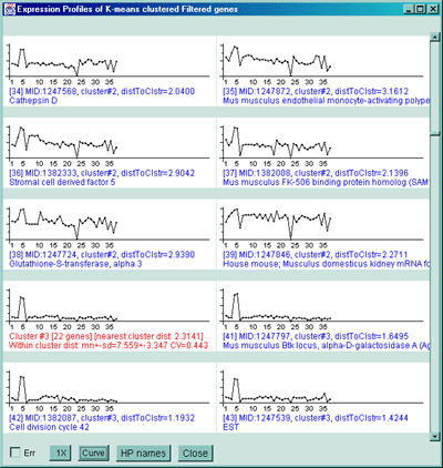
Figure 2.4.5.3 Genes clustered using the K-means cluster
method. A) Using the current gene as the initial cluster,
MAExplorer finds N orthogonal clusters assigning the set of filtered
genes to these clusters using the HP-E expression profiles. All
genes are iteratively assigned to these clusters. Genes belonging to
the current cluster are labeled with a green cluster number both in
the array and in the scatter plot. The slider determines the number of
clusters (set to 6 here). A 2D scatter plot shows the genes belonging
to cluster 6. The K-means cluster report on the right contains a sorted
list of the genes in each cluster and has buttons to generate EP
plots and reports as well as summary mean EP plots (shown) and mean
cluster reports. The detailed list is shown below. B) Part of
the scrollable EP plots for this data showing genes belonging to both
clusters #5 and #6. C) The mean EP plots for the 6 clusters.
Cluster report for 6 K-means clusters with 141 genes being clustered.
The seed gene is [1248564] Jun-B oncogene.

Clone ID  Similarity      Cluster-#  Distance-to-cluster  Gene-Name
--------  --------------  ---------  -------------------  ----------------

1248411   **************  1          Cluster [26 genes] in cluster [distNext: 1.035] wiCdist:mn+-sd=1.223+-0.453 CV=0.371  Calpactin I light chain
1381592   **********      1          0.448  Surfeit gene 4
1247956   *********       1          0.706  Protein kinase, cAMP dependent, catalytic, beta
1381836   ********        1          0.761  Prohibitin
1382325   ********        1          0.771  M.musculus mRNA for C1D protein
1248270   ********        1          0.775  Seven in absentia 1A
1247716   ********        1          0.794  Lipoprotein lipase
1248184   ********        1          0.847  Mus musculus bromodomain-containing protein BP75 mRNA, complete cds
1248564   *******         1          0.864  Jun-B oncogene
1382667   *******         1          0.888  SERINE/THREONINE PROTEIN PHOSPHATASE PP2A-BETA, CATALYTIC SUBUNIT
1382561   *******         1          0.931  Mus musculus GTP-specific succinyl-CoA synthetase beta subunit (Scs) mRNA, partial cds
1248089   ******          1          1.013  M.musculus RPS3a gene
1247780   ******          1          1.088  Proprotein convertase subtilisin/kexin type 7
1247557   ******          1          1.104  M.musculus L28 mRNA for ribosomal protein L28
1248321   *****           1          1.278  Decay accelerating factor 1
1382751   ****            1          1.311  Clusterin
1382007   ****            1          1.357  Murine mRNA with homology to yeast L29 ribosomal protein gene
1382074   ****            1          1.390  Orosomucoid 1
1381963   ****            1          1.417  M.musculus mRNA for ribosomal protein L36
1248278   **              1          1.658  HISTONE H3.3
1247630   **              1          1.675  Procollagen, type I, alpha 2
1247865   *               1          1.837  Mouse beta-D-galactosidase fusion protein mRNA, complete cds
1382236   *               1          1.85  Caspase 7
1247833                   1          1.882  Mus musculus radio-resistance/chemo-resistance/cell cycle checkpoint control protein (Rad9) mRNA, complete cds
1248535                   1          1.953  M.musculus mRNA for selenoprotein P
1247702                   1          2.157  Cytochrome C oxidase, subunit Va
1382282   **************  2          Cluster [13 genes] in cluster [distNext: 24.199] wiCdist:mn+-sd=16.184+-6.667 CV=0.412  Max interacting protein 1
1382159   **********      2          9.086  TRANSPLANTATION ANTIGEN P35B
1247854   *********       2          11.002  Prolyl 4-hydroxylase, beta polypeptide
1247970   ********        2          11.786  Mouse mRNA for osteoblast specific factor 2 (OSF-2)
1381663   ********        2          12.948  Mus musculus vacuolar adenosine triphosphatase subunit A gene, complete cds
1382100   ********        2          13.34  T-complex protein 1, related sequence 1
1248366   ********        2          13.541  Mus musculus cytochrome c oxidase subunit VIIa-L precursor (Cox7al) mRNA, nuclear gene encoding mitochondrial protein, complete cds
1247568   ********        2          13.762  Cathepsin D
1247872   *******         2          14.015  Mus musculus endothelial monocyte-activating polypeptide I mRNA, complete cds
1382333   *******         2          14.065  Stromal cell derived factor 5
1382008   *******         2          15.985  Mus musculus FK-506 binding protein homolog (SAM11) mRNA, complete cds
1247724   ****            2          21.964  Glutathione-S-transferase, alpha 3
1247846                   2          34.704  House mouse; Musculus domesticus kidney mRNA for Phosphatidic acid phosphatase, complete cds
1247945   **************  3          Cluster [22 genes] in cluster [distNext: 11.979] wiCdist:mn+-sd=7.559+-3.347 CV=0.443  Mus musculus mRNA for DEDD protein
1247797   **********      3          4.159  Mus musculus Btk locus, alpha-D-galactosidase A (Ags), ribosomal protein (L44L), and Bruton's tyrosine kinase (Btk) genes, complete cds
1382087   **********      3          4.494  Cell division cycle 42
1247539   **********      3          4.511  EST
1248212   **********      3          5.009  Murine mRNA for integrin beta subunit
1248470   **********      3          5.044  EST
1247521   *********       3          5.299  Mus musculus mRNA for peroxisomal integral membrane protein PMP34
1381808   *********       3          5.924  Mus musculus UDP-GalNAc:polypeptide N-acetylgalactosaminyltransferase-T3 mRNA, complete cds
1381970   *********       3          6.285  Mus musculus thioredoxin mRNA, nuclear gene encoding mitochondrial protein, complete cds
1382168   *********       3          6.343  N-terminal Asn amidase
1382704   *********       3          6.36  Mus musculus N-myristoyltransferase 1 mRNA, complete cds
1248548   *********       3          6.378  Mus musculus WDR protein mRNA, complete cds
1247564   ********        3          6.652  Erythrocyte protein band 7.2
1248588   ********        3          6.67  M.musculus BAP31 mRNA
1247541   ********        3          6.690  Apolipoprotein D
1248462   ********        3          7.322  Sterol O-acyltransferase 1
1248462   ********        3          7.42  Sterol O-acyltransferase 1
1248521   ******          3          9.121  Mus domesticus nuclear binding factor NF2d9 mRNA, complete cds
1382212   ******          3          10.137  Thyroid autoantigen 70 kDa
1382270   *****           3          10.529  Voltage-dependent anion channel 2
1248152   *****           3          10.541  M. musculus mRNA for MAP kinase-activated protein kinase 2
1247678                   3          19.431  Casein alpha
1247543   **************  4          Cluster [44 genes] in cluster [distNext: 1.035] wiCdist:mn+-sd=0.439+-0.266 CV=0.606  RAS-related C3 botulinum substrate 1
1381923   ************    4          0.158  Prolyl 4-hydroxylase, beta polypeptide
1382052   ************    4          0.209  Trans-acting transcription factor 1
1247882   ***********     4          0.237  Mus musculus AMP activated protein kinase mRNA, complete cds
1248099   ***********     4          0.246  Mus musculus mitogen-responsive 96 kDa phosphoprotein p96 mRNA, alternatively spliced p67 mRNA, and alternatively spliced p93 mRNA, complete cds
1248351   ***********     4          0.251  Abl-interactor 1
1247540   ***********     4          0.255  Mus musculus mRNA for ZIP-kinase, complete cds
1248316   ***********     4          0.26  Mus musculus proteasome alpha7/C8 subunit mRNA, complete cds
1382671   ***********     4          0.264  Mouse MA-3 (apoptosis-related gene) mRNA, complete cds
1382014   ***********     4          0.277  Transcription elongation factor B (SIII), polypeptide 1 (15 kDa),-like
1247885   ***********     4          0.289  Mus musculus mRNA for ryudocan core protein, complete cds
1248294   ***********     4          0.292  Mus musculus thioredoxin-related protein mRNA, complete cds
1382066   ***********     4          0.306  Inhibitor of DNA binding 2
1248597   ***********     4          0.307  Lipocortin 1
1248591   ***********     4          0.324  Interferon beta, fibroblast
1248445   **********      4          0.333  Mus musculus beta prime coatomer protein mRNA, partial cds
1247775   **********      4          0.34  House mouse; Musculus domesticus male brain mRNA for ARF1, complete cds
1382750   **********      4          0.340  Thymoma viral proto-oncogene
1247905   **********      4          0.341  Monokine induced by gamma interferon
1381668   **********      4          0.351  Mus musculus mitogen-activated protein kinase-activated protein kinase mRNA, complete cds
1381811   **********      4          0.356  Protein tyrosine phosphatase, receptor type, D
1382031   **********      4          0.358  Protease (prosome, macropain) 28 subunit, beta
1248345   **********      4          0.363  Mus musculus alpha-methylacyl-CoA racemase mRNA, complete cds
1382555   **********      4          0.364  Lysosomal membrane glycoprotein 1
1247820   **********      4          0.367  Tight junction protein 1
1247598   **********      4          0.374  Retinoblastoma 1
1247595   **********      4          0.378  PROBABLE CALCIUM-BINDING PROTEIN PMP41
1381928   **********      4          0.379  Mus musculus MRJ (Mrj) mRNA, complete cds
1248196   **********      4          0.399  Max protein
1381691   **********      4          0.423  SRY-box containing gene 17
1248225   **********      4          0.434  Mus musculus heat shock transcription factor 1 (Hsf1) gene, partial cds
1248084   **********      4          0.442  Mus musculus Supl15h gene
1247941   *********       4          0.453  Fibroblast growth factor inducible 14
1381623   *********       4          0.468  Stearoyl-coenzyme A desaturase 1
1248202   *********       4          0.473  Mouse mRNA for PAP-1, complete cds
1382115   *********       4          0.512  GLUTATHIONE S-TRANSFERASE GT8.7
1382044   *********       4          0.515  Cartilage derived retinoic acid sensitive protein
1381636   ********        4          0.567  Lymphotoxin B
1381920   ********        4          0.569  Mus musculus mRNA for NEFA protein, complete cds
1247757   ********        4          0.596  Granzyme B
1382094   ********        4          0.609  High mobility group protein 1
1247545   ********        4          0.638  Carbon catabolite repression 4 homolog (S. cerevisiae)
1247607   ***             4          1.188  POLYADENYLATE-BINDING PROTEIN
1247727                   4          1.667  Malate dehydrogenase, mitochondrial
1248244   **************  5          Cluster [19 genes] in cluster [distNext: 3.473] wiCdist:mn+-sd=4.273+-2.059 CV=0.482  CD80 antigen
1248534   **********      5          1.648  Carbonyl reductase
1247764   **********      5          1.776  H-2 CLASS II HISTOCOMPATIBILITY ANTIGEN, GAMMA CHAIN
1381933   *********       5          2.345  Mouse rpS17 mRNA for ribosomal protein S17, complete cds
1381616   *********       5          2.42  Mus musculus oral tumor suppressor homolog (Doc-1) mRNA, partial cds
1248232   *********       5          2.486  Mus musculus putative glycogen storage disease type 1b protein mRNA, complete cds
1382644   ********        5          2.717  Cyclin G
1248125   ********        5          2.791  Histocompatibility 2, class II, locus Mb2
1247799   ********        5          2.869  Mus musculus signal recognition particle receptor beta subunit mRNA, complete cds
1247708   ********        5          3.024  Ephrin A1
1247932   ******          5          4.235  Mus musculus (clone: pMAT1) mRNA, complete cds
1382515   *****           5          4.668  ATPase, Na+/K+ beta 3 polypeptide
1248586   *****           5          4.838  Mus musculus viral envelope like protein (G7e) gene, complete cds
1248198   ***             5          5.874  Mus musculus D9 splice variant 2 mRNA, complete cds
1381623   **              5          6.224  Stearoyl-coenzyme A desaturase 1
1382086   *               5          6.885  Mus musculus (strain C57Bl/6) mRNA sequence
1247887   *               5          7.014  Mouse chromosome 6 BAC-284H12 (Research Genetics mouse BAC library) complete sequence
1247886                   5          7.810  Cut (Drosophila)-like 1
1248303                   5          8.094  Lipopolysaccharide response
1247621   **************  6          Cluster [17 genes] in cluster [distNext: 19.157] wiCdist:mn+-sd=12.410+-3.024 CV=0.244  Mus musculus Lsc (lsc) oncogene mRNA, complete cds
1248050   *******         6          7.407  Mus musculus C57BL/6J ribosomal protein S28 mRNA, complete cds
1247698   *******         6          7.571  Adipocyte protein aP2
1248240   *****           6          9.198  Mus musculus mRNA, complete cds
1247862   ****            6          9.844  Mus musculus Nmi mRNA, complete cds
1382162   ****            6          10.330  CAMP responsive element modulator
1248398   ***             6          11.007  Mouse mRNA for ribosomal protein S12
1248281   ***             6          11.143  M.musculus mRNA for histone H3.3A
1247852   ***             6          11.576  Twist gene homolog, (Drosophila)
1381991   **              6          12.809  Prolyl 4-hydroxylase, beta polypeptide
1382753   **              6          13.019  Mus musculus cleavage and polyadenylation specificity factor (MCPSF) mRNA, complete cds
1248368   *               6          13.639  Mus musculus ribosomal protein S26 (RPS26) mRNA, complete cds
1247639   *               6          13.692  SRY-box containing gene 4
1248435                   6          14.262  Thymus cell antigen 1, theta
1247961                   6          14.75  ATP SYNTHASE ALPHA CHAIN, MITOCHONDRIAL PRECURSOR
1248344                   6          15.217  Gut enriched Kruppel-like factor
1382234                   6          16.351  CD8 antigen, beta chain
We call the genes closest to the "center" of the K clusters primary
genes and they are reported with additional information. The "Cluster
[# genes]" entries in the distance-to-cluster fields indicates that
these genes are the center of the clusters (i.e. primary genes). The
distNext is the distance from this cluster center to the next nearest
K-means cluster center. The number of clusters N (6 in this example)
is set in the popup state scroller. If you change the value of N, it
will recompute the clusters and the primary genes.
It draws magenta circles around the
primary genes in the microarray and the cluster number to the right of
the circle. The size of a circle corresponds to the number of genes
clustered with that circle. If you click on a gene belonging to any
cluster, it defines that cluster as the "current cluster". It will
change the labels of the subset of genes that belong to the current
gene from red (white) circle to a green (yellow) cluster number of the
current cluster in the intensity (ratio) pseudoarray image. In addition,
the 'edited gene list' is set to the subset of genes that belong to
the current cluster. If you are also displaying a scatter plot, genes
in the current cluster have their red '+' characters changed to the
cluster number.
You can click on that gene in the array image to determine its
identity. You may also popup an ordered (same as the above report)
plot of the clusters expression profiles by clicking on the EP
plot button. You may plot the mean expression profiles of the N
clusters using the Mean EP plot button. You may generate a
report of all of the clustered genes or of the mean clusters using the
Cluster-Report or Mn-Cluster-Report buttons
respectively. If you change the Filter conditions, you may recompute
the clusters using the Recompute Clusters button. Closing the
text window will remove the magenta
circles. If you selected the current cluster, the genes that
belong to it will still be available in the 'edited gene list' for
making reports, saving as a gene subset or for additional gene
filtering. If you press the SaveAs GeneSets button, then K gene
sets are created with the names "Cluster#1", "Cluster#2", ...,
"Cluster#K". You can then save or rename the clusters you want and
delete the rest. If you press the ClusterGram button, it
displays the gene sets in a cluster gram order the same way as
the cluster report.
The Hierarchical clustering of expression profiles computes the
hierarchical clustering of the expression profiles of data Filtered
genes and displays a clustergram and optional dendrogram.
Hierarchical clustering is described in ( Sneath and Sokol, 1973). The gene
data is normalized either by the corresponding HP-X sample data for
each gene or the maximum raw intensities for each HP sample in the
expression profile set by the Normalize by HP-X else HP's max
intensities menu toggle. There are three types of clustering
linkages: average-arithmetic-linkage,
average-centroid-linkage, and next minimum
linkage. These may be modified using the weighted average
that gives equi-weighting to the child clusters in computing the mean
of a new cluster, and un-weighted-average that weights them by
the number of non-terminal clusters. The average-linkage clustering is
very compute intensive and takes a while. The next-minimum-linkage is
much faster and may result in adequate clustering for some
situations.
Clustering is represented by a binary tree and is visualized as an
ordered gene clustergram and optional dendrogram sub-plot. This is
similar to the methods of (DeRisi,
1996), (Eisen, 1998), and
(White, 1999). Currently,
MAExplorer does 1-way clustering - not the 2-way clustering of (Weinstein, 1998) and (Eisen, 1998). Each row of the
clustergram represents a gene and each column represents a HP in the
HP-E list of samples. Each box in a row represents the normalized
expression of that gene for the HP represented in that column. The
color of the box is one of 9 colors representing the normalized
expression ranges and assigned according to the following table:
Table 2.4.5.4. ClusterGram pseudocolor assignments. The
colors are assigned to "box" entries in the clustergram corresponding
to genes. The color represents data as either the X/Y ratio or X-Y
Zdiff relative to the normalizing HP.
| . |
. |
. |
. |
. |
. |
. |
. |
. |
| bright green |
. |
. |
dark green |
Black |
dark red |
. |
. |
bright red |
| <1/8X |
1/6X |
1/4X |
1/2X |
1X |
2X |
4X |
6X |
>8X |
The current gene may be set by clicking on a row that is then
highlighted in green. If you click on a colored box, it will also
report the HP name for that column and its normalized expression value
(highlighting that box with a white circle). If the Web genomic
databases are enabled (through the View menu, then it will also popup
a Web page for that gene). If you set the current gene in any of the
array, scatter plot, gene guesser, etc. displays, it will set it for
and position the clustergram at that gene. If the Dendrogram
checkbox is enabled, then a dendrogram is drawn to the left of the
clustergram boxes. Clicking on a region in the dendrogram sets a
distance threshold (displayed at the top) and displays all parts of
the dendrogram tree in red that have a cluster distance less than what
you defined. If the zoom nnX button is pressed, then the
of dendrogram drawing is magnified by nnnn-fold to make highly similar
clusters more visible. Pressing the button repeatedly cycles through:
1X, 2X, 5X, 10X, 20X. Sub-regions of the clustergram may be explored
in more detail using the EP plot button that pops up a
scrollable window of the ordered gene list. You may generate
multiple EP-subset plots so as to compare different parts of the
clustergram. A report of all of the ordered genes may be created
using the ClustGram Report button. The Show HP names
button pops up a numbered list of all samples used in the expression
profiles and clustergram. This report has all of the normalized
expression profiles on the right side of the report.
A)
B)
C)
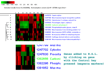
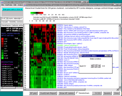
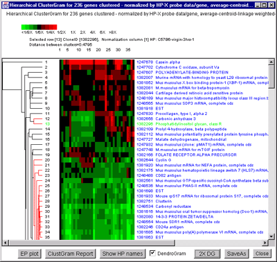
Figure 2.4.5.4 Hierarchical clustering clustergram of genes
filtered by ratio histogram bins for 19 samples from the MGAP data
set. The hybridized samples are drawn as colored boxes in the 19
columns. Rows of boxes correspond to gene expression profiles. In
A), the set of all genes and ESTs was filtered by the CV filter
set to 0.387 and the normalization was the Zscore. The gene "Mus
musculus D9 spice variant 2 mRNA, complete cds" was selected as the
current gene in the clustergram. Data for this gene and the selected
HP column is indicated at the top of the clustergram. The list of the
19 samples is shown on the left. B) Details of clustergram and
dendrogram are shown where the user had selected a cluster distance
threshold at "Mouse mRNA for mitochondrial cytochrome c oxidase
subunit Vb" in the dendrogram part of the plot (zoomed by 2X). This
selection draws all parts of the dendrogram tree that are less than
this distance are drawn in red. C) shows the manual selection
of genes from the ClusterGram or Dendrogram by clicking on the genes
names you wish to capture in the Edited Gene List (EGL) while the
Control key is pressed. The zoomed subregion shows three genes in the
same cluster that were selected (magenta stars in the right edge of
the ClusterGram).

MAExplorer - Microarray Exploratory Data Analysis
Various reports summarizing gene or sample data may be generated and
appear in popup tables. These include:
- Data on all of the hybridized samples in the database
including links to related Web databases
- Data on additional quantification and descriptive information
on the hybridized array samples in the database
- Hybridized sample calibration, Samples vs. Samples correlation
coefficient of Filtered genes, and mean & variance tables
- Tables of all named genes, the calibration DNA genes, etc.
- A table of genes in the 'Edited Gene List'
- A table of genes in the current Gene Class
- A table of genes passing the "Filter"
- The N genes with the highest or lowest ratios (HP-X/HP-Y
or F1/F2) of the Filtered genes (N defaults to 100, but may
be changed as a Preference)
- Tables of additional data for the Filtered genes including
expression profile ratios, HP-X vs. HP-Y 'set' statistics if
the data is enabled for using HP-X and HP-Y 'set' data. If
you are doing a t-test of Kolmogorov-Smirnov test, then it
reports the p-value and test statistics.
- Table of statistics on F-test on the current Ordered
Condition List of samples/condition, including p-value and
F-test statistics.
- Tables of correlation coefficient statistics of data Filtered
genes comparing all samples in the HP-E list against each other.
- Tables are presented as either: a) an active
"clickable" spreadsheet that may contain links to Web sites
and pops up a Web browser window to that site (e.g.
histology links or model system in the array report), or
display additional gene features and numeric
comparisons. b) tab-delimited text that may be "cut"
and then "pasted" into an Excel type spreadsheet for further
analysis.
- Additional expression profile data (from the HP-E samples)
and/or statistical data from the HP-X vs. HP-Y 'sets' may
be included in gene report tables.
- Clicking on a column name in the dynamic report will
sort the report by data in the report in ascending and
descending order.
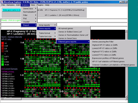
Figure 2.4.6 Reports menu. You may create either dynamic or
tab-delimited text reports of either Samples or of subsets of genes.
These may be presented as interactive dynamic tables as well as
scrollable text windows capable of being exported to Excel. If Web DB
access is enabled, clicking on an entry will bring up a Web browser
with access to GenBank data. If the report contains Clone ID as one
of the fields, you can click on it to have it define that gene as the
current gene and highlight it in the microarray image or scatter plot
(if it is being used). The reports are divided into two types - those
dealing with lists of arrays (i.e. the sample experimental condition)
and those dealing with lists of genes.
The Report menu includes:
-
Array reports
 -
show tables of sample array information.
-
Gene reports
 -
show tables of sets of genes information.
- --------------------
-
Table format
 - generates the
table as 'Spreadsheet', 'Tab delimited', or 'Name=Value list'.
-
Table font size
 - changes
the report font size from default 10 point.
You may generate reports of sample array information. The first two
menu selections contain descriptive information about specific
hybridized microarrays samples. The "Extra Samples info" contains
quantitative and extra descriptive information (if available for your
database).
The "Samples vs Samples correlation coefficients" computes the correlation
coefficients in an upper diagonal matrix for the current set of
Filtered genes showing HP samples similarity. Then entries are of the
following form where HP:1 and HP:2 correspond to samples listed in the
field names of the table and the data is the intensity values using
the current normalization method.
rSq=0.748, n=1656, HP:1(mn+-sd)=(28991+-19564), HP:2(mn+-sd)=(5044+-9766)
The "Calibration DNA summary" table contains the computed means,
std-dev, and computed normalization scale factor for all active
hybridized samples. The scale factors are used if the 'Calibration
DNA' normalization is used.
You must set the Web access checkbox if you want to click on a blue
hyperlink in the resulting report to access an associated Web
database.
- Samples info - show table of all samples accessible in
the database.
- Samples Web links - show table of Web links for all
sample samples accessible in the database.
- MAE Projects DB - show table of project databases if the
project startup database exists (stand-alone mode).
- Extra info on Samples - show table of
additional information on all of the samples in the database.
- Sample vs Sample correlation coefficients - show table of
correlation coefficients for all HP-E selected samples for genes
meeting the data Filter criteria.
- 'Calibration DNA' summary - show a table of means, std-dev,
scale factor for all HP-E selected samples.
- HP mean & variance summary - show table of means,
std-dev, min, max, etc. of raw intensity data for all HP-E selected
samples.
A)
B)
C)
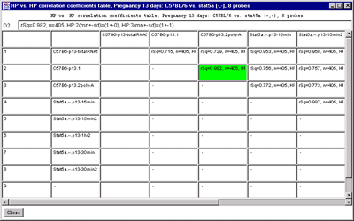
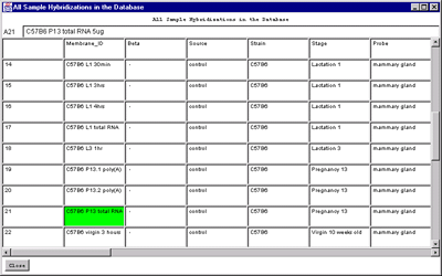
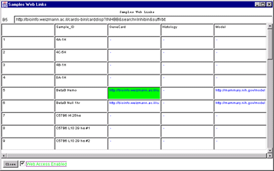
Figure 2.4.6.1 Hybridized samples dynamic Report windows. A)
Samples Info report. B) Sample Web links. Clicking on a blue
hypertext link brings up the corresponding genomic Web database entry
in a separate Web browser window if the Web access is enabled. The
tab-delimited version of the same reports (not shown) may be cut and
then pasted into other programs such as an Excel spreadsheet.
C) HP vs HP correlation table on genes passing the data
Filter for all samples in the HP-=E list.
You may generate gene reports with various additional options. You
must set the Web access checkbox if you want to click on a blue
hyperlink in the resulting report to access an associated Web
database. In addition, specialized gene reports may be generated from
some of the cluster plot command windows. These include lists of
genes sorted by cluster (K-means cluster #), by hierarchical cluster order,
by similarity to a gene, etc. The mean cluster expression values may
be reported for K-means clustering.
- All named genes - show table of all genes where the gene
is named.
- Genes in 'Edited Gene List' - show table of genes in the
'Edited Gene List'.
- Genes in 'Normalization Gene List' - show table of genes in the
'Normalization Gene List'.
- Genes in GeneClass - show table of genes in the current
gene class.
- Filtered gene reports
 - show genes
that meet the data Filter criteria.
You may generate gene reports of Filtered genes with various
additional presentation options. In the highest/lowest N genes, N
defaults to 100 and is set by (Report | Table format | Set max # genes
in highest/lowest report) command.
- Genes passing the Filter - all genes passing the Filter
- Highest HP-XY ratios or Zdiff - top N Filtered genes
- Lowest HP-XY ratios or Zdiff - lowest N Filtered genes
- Highest F1/F2 ratios or Zdiffs - top N Filtered genes (if
duplicates). If ratio data, then highest Cy3/Cy5
- Lowest F1/F2 ratios or Zdiffs - lowest N Filtered genes
(if duplicates). If ratio data, then lowest Cy3/Cy5.
- Expression profiles Filtered genes - show numeric
expression ratios for HP-E data scaled to the first HP in HP-E.
- HP-XY 'set' statistics of Filtered genes - show
(mean,stdDev,CV,n) data for both the HP-X and HP-Y
sets. If the t-Test is active, also show (p-value, df,
t-statistic, pF-sameValue). If the Kolmogorov-Smirnov test is
active, then it reports the (p-value, df, D-statistic).
- Ordered Condition list statistics of Filtered genes - for
the current OCL if the F-test is active, show the (f-statistic,
dfWithin, dfBetween, mnSqWithin, mnSqBetween)
(mean,stdDev,CV,n) data for each condition.
If Cy3/Cy5 ratio data is being analyzed, then the Highest (Lowest)
F1/F2 entries become
- Highest Cy3Cy5 ratios or Zdiffs - top N Filtered genes (if duplicates)
- Lowest Cy3Cy5 ratios or Zdiffs - lowest N Filtered genes (if duplicates)
A)
B)
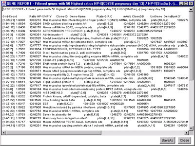
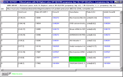
Figure 2.4.6.2 Gene Report windows of 50 named genes with highest
HP-X/HP-Y 'set' ratios. A) Dynamic gene report of 50
genes with highest HP-X/HP-Y 'set' ratios. A similar report may be
generated for the lowest ratios or for single HP-X/HP-Y samples. This
type of report may be generated for the highest or lowest Zdiff values
when the Zscore normalizations are used. Clicking on a blue hypertext
link brings up the corresponding genomic Web database entry in a
separate Web browser window if the Web access is enabled. It also sets
the current gene to the gene for that row. B) The
tab-delimited version of the same report may be cut and then pasted
into other programs such as an Excel spreadsheet.
The report is presented as a table. However, it may be visualized
several different ways. The scrollable spreadsheet includes the
ability to click on blue hypertext items and have a Web browser pop up
for that item on a Web database (e.g. GenBank, dbEST, UniGene,
LocusLink, mAdb Genes, GeneCard, etc). The tab-delimited option
enables you to cut the table and paste it into a separate spreadsheet
program such as Excel. You may also extend the data in the table to by
'Adding' expression profile ratios and statistics from the HP-X and
HP-Y 'set' comparisons.
-
 Spreadsheet [RB] - some cells (indicated by blue) are
connected Web databases that are accessed by clicking on them (default).
-
 Tab delimited - suitable for export [RB] - as in Excel, etc.
- --------------------
-
 Set max # genes in highest/lowest report or filter [CB] -
sets the number of genes N to report or use in data Filter.
-
 Add EP data to Gene-Reports [CB] - for each of the
samples in HP-E.
-
 Use EP data in Gene-Reports [CB] - use raw EP data (under
the current normalization) else use data normalized to
0.0 to 1.0 by maximum value for all genes being displayed.
-
 Add HP-X/-Y 'set' statistics data to Gene-Reports [CB] -
that includes (mean,stdDev,CV,n) for both the HP-X and
HP-Y sets.
For wider tables, you can see more information if you use a smaller
font to display the table. The font sizes available are:
-
 12pt [RB]
-
 10pt [RB] - (the default size)
-
 8pt [RB]

MAExplorer - Microarray Exploratory Data Analysis
The View menu options are used to modify the view of genes
visible in the pseudoarray image. Genes may be displayed with
additional properties or capabilities including access to Web-based
genomic database entries for specific genes. Note that depending on
your particular database, if some genomic identifiers are not
available then the corresponding "Enable display current gene in
genomic DB Web browser" will not appear in the menu.
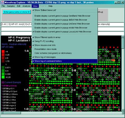
Figure 2.5 View Menu options. These are divided into various
options for modifying the presentation as well as recording activity
such as the messages or history popup scrollable log windows.
-
 Show 'Edited Gene List' [CB]
- toggle showing the EGL as magenta boxes in the pseudoarray
image. If enabled, genes set by manual selection or as the
result of some filtering operations (see Edit menu, the
Filter and Clustering)
- ----------------------
-
 Enable display current
gene in GenBank Web Browser [RB] - when click on a gene in
microarray image or scatter plot to access NCBI data. It will
use RefSeqID data if available.
-
 Enable display current
gene in dbEST Web Browser [RB] - when click on a gene in
microarray image or scatter plot to access NCBI data.
-
 Enable display current
gene in Unigene Web Browser [RB] - when click on a gene in
microarray image or scatter plot to access NCBI data.
-
 Enable display current
gene in mAdb Web Browser [RB] - when click on a gene in
microarray image or scatter plot to access NCI/CIT data.
-
 Enable display current
gene in LocusLink Web Browser [RB] - when click on a gene in
microarray image or scatter plot to access NCBI LocusLink data
(by Locus ID if available, and GenBank ID if it] is not).
-
 Enable display current
gene in OMIM Web Browser [RB] - when click on a gene in
microarray image or scatter plot to access NCBI OMIM data by
OMIM ID if available.
- ----------------------
-
 Show Filtered spots in array
[CB] - if on, show Filtered genes in the microarray image
using circle overlays just outside of each spot. Genes not
passing the Filter have no circle.
-
 Gang F1-F2 scrolling
[CB] - toggle gang scrolling. If on, gang measure F1 and F2
when click on one of them. If off, only measure only the spot
that you click on.
-
 Show mouse-over info
[CB] - toggle mouse over. If enabled, report HP or gene
details when the mouse is moved over the sample names or spots
in the array image or genes in scatterplot or expression profile
overlay plot.
-
 Presentation view mode
[CB] - toggle presentation mode. If enabled, increase the
fonts to 12pt and draw darker circles, squares, and "+" so the
display details are easier to see when projecting the display or
making slides.
-
 Color scheme (red-green) or
dichromasy [CB] - toggle between two color schemes red-green
and orange-blue for dichromasy which may be easier for some
people.
-
 Show log of messages
[CB] - toggle message logging mode. If on, it pops up a
scrollable log of all messages to the three line status
area. This is useful for recording measurements and other
activity. The messages may be saved in log file.
-
 Show log of command history
[CB] - toggle command history logging mode. If enabled, it
pops up a scrollable history of all commands issued to
MAExplorer. The commands are automatically numbered. This is
useful for recording what steps you took during an analysis.
The history may be saved in log file.
A)
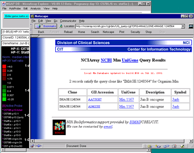
B)
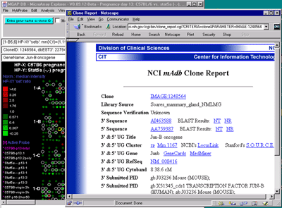
C)
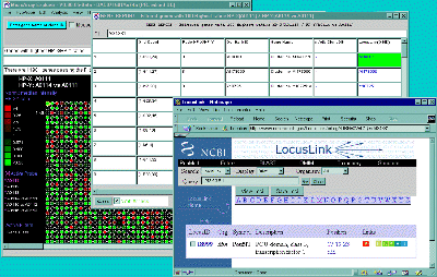
Figure 2.5. Popup genomic browser database page. A) The
UniGene Web page pops up in a new Web browser window when the user
clicks on a gene in the array image, 2D scatter plot or Report and the
view is set to "Display current gene in Unigene Web Browser" toggle
was enabled in the View menu. The current gene was "Jun-B oncogene".
Alternatively, the B) mAdb Gene DB may be selected - as well as
GenBank or dbEST genomic databases. C) Alternatively, data from
the NCBI LocusLink database may be accessed if either the GenBank ID or
LocusID is available.
2.5.1 Logging MAExplorer messages
MAExplorer shows various data measurements as well as many other types
of information in the three text lines in the status area of the main
window. The Show log of messages pops up a scrollable log of
all messages to the three line status area. This is useful for
recording measurements and other activity. The messages may be saved
in log file (typically maeMessages.log). Figure 2.5.2 shows an example
of the messages popup log window. Clicking on genes in the pseudoarray
image or in plots will log the gene data (see Section 3.3) given the
current normalization, Samples use (single or multiple), and
pseudoarray display mode. The current values of all of the State
Threshold scrollers are saved in the message log when the (Edit menu |
Preferences | Adjust all Filter threshold scrollers) State
Thresholds popup window is closed. This is useful for capturing the
current settings at any time.
2.5.2 Logging command history
During a datamining session, the user will typically execute many
commands from the menu as well as clicking on genes in the pseudoarray
image or in plots. It is useful to recording the steps you took during
this analysis. The Show log of command history pops up a
scrollable history of all commands issued to MAExplorer. The commands
are automatically numbered. The history may be saved in log file
(typically maeHistory.log). Figure 2.5.2 shows an example
of the command history popup log window.
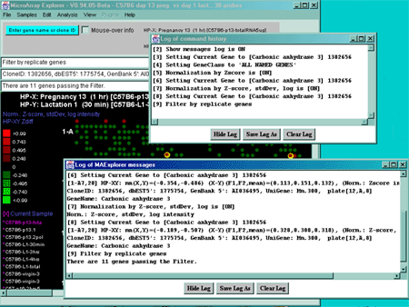
Figure 2.5.2 Examples of messages and command history popup log
windows. Measurements and other activity are shown in more detail
in the messages window whereas the command history indicates commands
(numbered in the order they are executed) in the command history window.
Data from either of these windows may be saved in text log files.

MAExplorer - Microarray Exploratory Data Analysis
MAExplorer may be extended by users to use new analysis methods using
Java plugins. We call these new methods MAEPlugins which are small
Java programs written by users that may be dynamically loaded into
MAExplorer and then applied to their data. These plugins will include
plugins written by LECB, those written by academic or commercial
groups. See the MAEplugins for
details. If you have a Java compiled plugin in the form of either a
Java .class or .jar file, you may load it at run time using the "Load
plugin" command in the Plugins menu. If specified in the MAEPlugin, it
will be added to the appropriate menu in the MAExplorer menu tree at
the end of the specified submenu (see Appendix C. Table C.5.7). If
this submenu "stub" is not specified, it will place in the list of
plugins in the Plugins menu (e.g. plugin #1, ..., plugin
#n).

Figure 2.6 MAEPlugins paradigm. If you have a MAEPlugin .jar
file, then it may be specified using the "Load plugin" command. When
you invoke the command from the menus (or other methods), it accesses
data from the current MAExplorer database it may need from the Open
Java API.
The Plugins menu includes:
- Load plugin - popup a browser to load a MAEPlugin jar file
- Unload plugin(s) - popup a selector to pick MAEPlugins to unload
- -------------------------------------
- RLO methods
 - list of
executable R methods (R LayOuts). These may be added by the user
using the RtestPlugin. An RLO
analysis allows you to export data from MAExplorer, execute it
with the R program, and import the R results back into
MAExplorer. [This is under development and is alpha-level.]
- Save RLO reports in time-stamped Report/ folder [CB] - puts files
generated by R from successive executions of the same RLO into separate
sub-folders in the Report/ folder with names
"RLOname-YYMMDD-HHMMSS/" to peep the data separate.
- -------------------------------------
-
- plugin #1 - 1st MAEPlugin added
- plugin #2 - 2nd MAEPlugin added
- . . .
- plugin #n - n'th MAEPlugin added
This contains a list of executable R
analyses methods (called R LayOuts or RLOs created with the
RtestPlugin) for evaluating MAExplorer data with R analysis scripts.
It is only available if you have installed the R language program (www.r-project.org) on your
computer. An RLO analysis allows you to automatically export data from
MAExplorer, execute it with the associated R program, and import the R
results back into MAExplorer. [This is under development and is
alpha-level.] A recent poster on
Extending MAExplorer with R is available as a PDF file.
The Save RLO reports in time-stamped Report/ folder [CB]
options puts files generated by R from successive executions of the
same RLO into separate sub-folders in the Report/ folder with names
"RLOname-YYMMDD-HHMMSS/" to peep the data separate. This is
useful when you want to compare results from the same RLO method but
with different MAExplorer preprocessing.
You may download the latest versions of all plugins using the (File |
Update Plugins from
maexplorer.sourceforge.net) menu command. Similarly, you can
update your versions of the RLO methods using (File |
Update RLO methods from maexplorer.sourceforge.net
This shows a short demonstration of what is involved in using a
MAEPlugin. The user first load the plugin from the disk. Generally the
plugins .jar or .class files are stored in the Plugins/ directory
where you have installed MAExplorer. Then they load a particular
plugin which installs it in the Plugins pull-down menu. Then they
revisit that menu to invoke the particular plugin. You may load any
number of plugins (until you run out of computer memory if that should
occur).
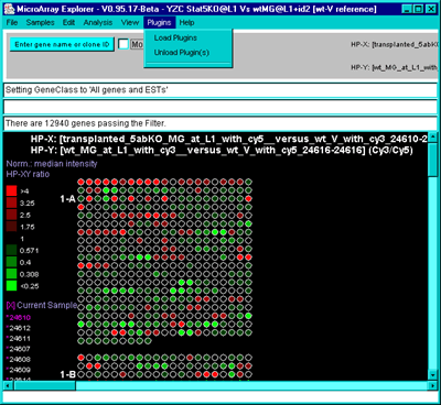
Figure 2.6.1 Loading a MAEPlugin from your file system using
the Load Plugins command in the Plugins pull down menu. If you
have a plugin .jar or .class file, it may be specified using the "Load
plugin" command. This pops up a file browser to let you specify the
plugin file.
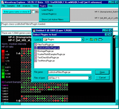
Figure 2.6.2 Executing the new command previously loaded in the
Plugin menu. Selecting the new "Show List Active Filters" command
that now appears in the Plugins menu invokes the plugin. This pops up
a report shown in the next figure.
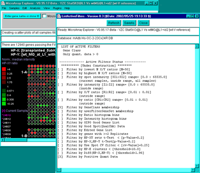
Figure 2.6.3 Popup window from executing the MAEPlugin.
This plugin gives a full report on the data Filter status in a new
pop up window.
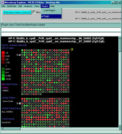
Figure 2.6.2 Plugins menu - executing a previously loaded
plugin. Plugins that do not go into particular MAExplorer
submenus go into the Plugins menu. Selecting the command will
invoke that MAEPlugin.

MAExplorer - Microarray Exploratory Data Analysis
Various on-line help and documents are available if you are connected
to the Internet. These will appear in a separate pop-up Web browser
window so you may view them while working with MAExplorer. This
includes on-line documentation (including this reference manual),
tutorials, and other information. This may be links to other Web pages
describing key areas of specific databases. For example, for the MGAP
database, the point back to key areas of MGAP including the MGAP Animal Models, Histology
atlas, etc. You can then use the browser's "Save as" and "Print"
options to save the data to a file or print it.
The Help menu includes:
- Home page - MAExplorer home page on SourceForge.net
- Introduction - to MAExplorer
- Overview - overview of MAExplorer capabilities
- Short tutorial - simple tutorial
of things to try in MAExplorer (Appendix A)
- Advanced tutorial - advanced tutorial
of things to try in MAExplorer (Appendix B)
- Menu summary - short summary of the MAExplorer menus.
- Reference manual - this Reference Manual document
- MAEPlugins - plugin home page for MAExplorer
- Intro to data mining - for MAExplorer, (Chapter 3)
- Glossary - glossary
of terms used in MAExplorer Reference Manual
- Index - Index
of terms used in MAExplorer Reference Manual
- -------------------------------------
-
Database-specific help menu entries -
entries defined for a particular database (see below)
|
- -------------------------------------
- About - show MAExplorer authors, version and revision
date
2.7.1 Adding custom help links to your database to the Help menu
These Database-specific help menu
entries list of entries are keyed to the database you are
using and may be
customized by the database maintainer in the configuration file
(Section C.5.6) to links relating to the particular database. For
example, database specific help for the MGAP database is:
- List of hybridized samples - available from MGAP.
- MGAP animal models - animal models used in MGAP.
- MGAP home page - Mammary Genome Anatomy Program

MAExplorer - Microarray Exploratory Data Analysis
Data mining is the uncovering of relevant patterns of interest in data
from a particular problem domain (Tukey, 1977). Typically this
involves using various statistical techniques to identify the patterns
including cluster analysis. See
StatSoft Inc's, 2002 on-line statistics textbook for definitions of
clustering and other statistical terms. Researchers across a wide
range of fields such as (Tufte,
1997) and (Cleveland,
1985) have suggested that a major aspect of this problem is
finding the correct means of graphical presentation to allow humans to
be a part of the pattern recognition process. Tufte argues that the
proper display of quantitative data in the context of the problem
domain can aid in the understanding of complex sets of data. This
carries over to the analysis of microarrays with data mining involves
having statistical, genomic knowledge database, and graphical
components for success. (Jagota,
2001) discusses a number of methods and applications for
microarray data analysis and visualization. Other useful resources are
the sets of papers in (
"Chipping Forecast", Nature Genetics supplement, Jan,
1999), and (
"Chipping Forecast II, Nature Genetics supplement, Dec,
2002).
This section briefly addresses some of the issues you need to
consider. However, a full discussion of the issues involved is beyond
the scope of this manual. These issues are covered in other more
focused statistical methods literature and you might also address them
in consultation with biostatisticians. The Internet has vast resources
for microarrays. A few to get you started might include: a microarray
citation electronic library
http://arrayit.com/e-library/, the National Library of Medicine PubMed
journal search engine, a general microarray Listserv
GENE-ARRAYS@ITSSRV1.UCSF.EDU. The MGED group (Brazma, 2001) has published the MIAME
standard which specifies (Minimum Information About a Microarray
Experiment). This information is useful in doing an analysis. Also
try searching using general Internet search engines. There are a
number of public microarray data repositories. One that we find useful
is NCBI's GEO (Gene
Expression Omnibus), that contains array data and MIAME compliant
information about the arrays.
- Data mining is a pattern discovery activity - use all the tools
you have.
- It is open-ended because of the variety of ways data may be
partitioned, normalized, pre-filtered, clustered, and viewed. Patterns
that are apparent in one view may not be apparent in another.
- When data-mining microarray data, look at correlated genes from
the point of view of what relationships might be interesting from a
biological view by characterizing genes that cluster together using
additional information. I.e. check out the results with various NCBI
and PubMed database searches on the resulting genes, by designing
other lab experiments to better uncover the cause and effect,
etc. Remember correlation does not imply cause and effect.
Organization of Sections in this Chapter
3.7 describes how to export
(i.e. save) report and plot data to your local computer.
There are a number of objectives an investigator has when analyzing a
set of data. The types of analyses and how useful they are depends on
what they wish to get out of the analyses as well as the type of
data.
A good and appropriate experimental design (i.e. the design and
setting up of experiments to subsequently be analyzed) is critical for
resolving significant differences in gene expression between
experimental conditions. We touch on some of the issues here. (Simon, 2001), (Dudoit,2000), and Kerr and
Churchill (2001a, 2001b) discuss some of the issues
of experimental design for microarrays. We do not currently implement
the Kerr-Churchill method. However, some of the issues involved in experimental design based on the types
of arrays are discussed in Section 3.1.1 for (Cy3/Cy5)-labeled as well
as 33P-labeled samples.
If users are comparing two different types of samples, the analysis
would be different than if they were comparing an ordered sequence of
samples (e.g. time series, cell cycle, dose-response, tumor-stage,
etc.). MAExplorer gives users the ability to:
- Organize their experiments by sample characteristics allowing them
to perform a variety of mining analyses comparing gene expression
patterns between sets of different samples or comparing a single
sample within an array's set of genes.
- Explore, compare, and record these analyses and share the results
or intermediate data with other investigators.
- Use graphical direct-manipulation combined with statistical
methods, clustering and spreadsheet techniques to gain different
insights into the structure of the data.
- Access public Internet genomic databases for particular genes
that are found to be interesting.
Briefly, data mining is the discovery of potentially interesting
patterns in the data that were previously unknown. One approaches the
analysis of a set of data with minimal expectations. However, some
idea of what you are interested in helps focus the search. But beware
of the trap of mining the data until you get the results you hope
for. The following figure helps illustrate this process.

Figure 3.1 Flow chart of a typical data mining session. The
user makes some initial decisions on the experimental design such as
which hybridized samples to compare, the type and numbers of
replicates. They then make initial guesses as to the normalization
method to use, and the gene subset (the gene class) to concentrate on
when setting the data filter. The data is viewed in various modalities
to get a feeling for its inherent dynamic range and where interesting
outliers might appear. Clustering and plots helps bring these
differences into view. The results are then evaluated and either the
process is finished or the views are refined by adjusting data
normalization and filter parameters, data subsets to be investigated,
clustering methods, plots etc. and the process repeated until the user
is able to see the differences between gene subsets more clearly or no
significant differences appear to be found.
Obviously, this approach is a first approximation to what is
eventually required. But it does capture the flavor of the data-mining
process. Typically the user would refine the search using variations
of the data filters and might contrast (using gene sets and hybridized
sample condition lists operations) results found under one set of
conditions with those found under another set of conditions.
Because of the iterative nature of this process, you might want to
keep a record of the commands you have used or the messages and
measurements you have made. To do this you need to enable message and
command history logging. Go to the View pull-down menu and then select
the type of logging you want using the Show log of messages or the
Show log of command
history commands.
*** THIS SUBSECTION IS IN THE PROCESS OF BEING UPDATED ***
Proper experimental design of microarray experiments is critical to
successful use of microarray data. Several recent reports discuss some
of the key issues involved in various aspects of statistical analysis
of microarrays: (Radmacher,
2001), (McShane, 2001),
(Korn, 2001), (Simon, 2001), (Dudoit,2000).
If we have two samples HP-X and HP-Y with a common reference sample P
(e.g. Cy5P), then we would be comparing the HP-X
"intensity" Cy3X/Cy5X against the HP-Y
"intensity" Cy3Y/Cy5Y. Alternatively,
you can label Cy3 as the common reference sample P in which case just
swap Cy3 and Cy5 in these equations. If you are using a common
reference standard (i.e. Cy5X1) is the same sample
as Cy5Y1 eg. a pooled sample
Cy5P, then
 a)   (Cy3X/Cy5X1) / (Cy3Y/Cy5Y1)
becomes
 b)   (Cy3X/Cy3Y)
However, this new comparison is accompanied by additional noise
because of use of the two Cy5P intermediaries.
An alternative method would be to compute
(Cy3X/Cy5Y) directly. However, this too
has its own sources of error and other problems, namely that not all
genes are labeled symmetrically with the two dyes since different dyes
may have different sequence specific affinities due to a variety of
causes. For that reason, dye-swap experiments are often
done. I.e. the two samples would be run as
(Cy3X/Cy5Y) as well as
(Cy3Y/Cy5X). If one were to plot
(Cy3X/Cy5Y) against
1.0/(Cy3Y/Cy5X) and the data were
perfectly symmetric (which they are not) then one would expect
a straight line. That is generally not what you get in practice.
Another issue is that when you have a number of samples A, B, C, D,
..., N and wish to compare them, there are a number of alternate
experimental designs you can use with different resulting sets of
advantages and problems. If a common pooled Cy5P
sample P were used, then the following experiments would be done:
(Cy3A/Cy5P), (Cy3B/Cy5P), ... , (Cy3N/Cy5P)
This assumes that there is enough of the pooled sample P to be used
for all of the experiments - otherwise additional sources of
error would be introduced. MAExplorer is ideally used with this
common reference sample P.
It a common pooled sample is not used, then the experimental
design becomes more complicated - especially if dye-swap experiments
are performed for all samples. For N samples taken 2 at a time
(i.e. Cy3 and Cy5), then the number of experiments may be impossibly
large to perform for other than a very small N. Eg. for N of 3, the
number of experiments is 3 and 6 if dye swap experiments are also
performed. For N of 4, the number of experiments is 6 and 12. And
this is without doing any replicate experiments. If a reasonable
number of replicates is added, then this set of experiments becomes
even difficult to perform.
MAExplorer is currently not oriented to handling these large
combinatoric types of non-pooled sets of experiments. However, you do
have the ability to swap (Cy3,Cy5) data on an individual basis so you
could compute an average of data from dye-swap experiments - but
with the caveats or non-uniform labeling mentioned above.
[(Cy3X/Cy5Y) + 1.0/(Cy3Y/Cy5X)]/2
In general, this is probably not a very good estimate.
There are several ways to implement a data mining system on moderate
size databases. The first is that all computations are performed on a
Web server and the user's Web browser displays the results. The second
is download an applet from the Web server, get the data from the
Web server and do computations in the Web browser. A third way is do
download data from a Web server and run a local stand-alone program on
the data. MAExplorer can be run using both the second and third
ways. However, we encourage the use of the stand-alone paradigm as
having the best bandwidth and being the most robust.
The browser-based computation paradigm (as opposed to server-based) is
somewhat unusual. It keeps both the program and data on the server,
making user maintenance of the latest versions easier than if they had
to constantly upgrade the program or data. This also has the distinct
advantage of giving the user instantaneous feedback through rapid
visual and tabular views and the ability to more effectively navigate
the data since the analysis is done on their desktop computer. Because
it is easy to access reference data from other genomic sources
(e.g. UniGene, GenBank, NCI/CIT's mAdb clone DB, dbEST, GeneCard,
etc.), it can be accessed from their respective Web servers as needed.
Complex browser-based computations are used in other data mining or
intensive computation domains. With the increased bandwidth of the
Internet and compute power and memory of PCs approaching the Cray
supercomputers of the previous decade, this paradigm becomes even more
feasible. However there are limits to how well it scales because of
Web browser limitations. Appendix E.2
discusses these issues in more detail
The major focus of the MAExplorer is interactive data mining with an
emphasis on direct graphical and tabular manipulation of the data.
The investigator is able to interact with the system by clicking on
spots in the array image, points in graphic plots, cells in
spreadsheets, by manipulating threshold sliders or typing in gene
names/clone Ids. This level of interaction allows investigators to
search for and identify patterns of differences with greater ease than
with a more static graphic system since it is easier to test ideas by
"grabbing onto the data". For example, "what" is the identity of
"this" outlier I am pointing to in a scatter plot; "which" genes are
best clustered with "this" gene in this clustergram and are perhaps
co-regulated; "which" genes have expression ratios within the range of
the histogram bins to that I am pointing?
Direct user manipulation of data, as incorporated in MAExplorer, was
defined by (Schneiderman,
1997) who defends the position that the direct manipulation of data
in data mining is an extremely effective means to amplify human
creativity in understanding patterns. Schneiderman's dogma states
"overview first, zoom, and then filter details on demand" and favors
the use of "shallow search trees, slide controllers, and
information-right screens with tightly coordinated panel view of
data", (Beardsly,
1999). MAExplorer also uses many of these direct manipulation
principles. It was designed to run on the desktop computers with data
residing on the same computer and loaded into its memory for rapid
direct manipulation - for both the Web browser and stand-alone
versions.
MAExplorer was designed to do flexible exploratory quantitative data
analysis of gene data from microarray hybridized sample experiments.
Many of the data-mining concepts are derived from a system called GELLAB-II
(http://www.lecb.ncifcrf.gov/lemkin/gellab.html) that is a UNIX-based
stand-alone exploratory data analysis system for 2D protein gels over
multiple experiments (Lipkin and
Lemkin, 1981), a review (Lemkin
and Lester, 1989) and examples of graphical representations of
this type of data (Lemkin,
1995). An on-line
GELLAB-II Web-Poster
(http://www.lecb.ncifcrf.gov/lemkin/gellab-ep93wd.html) is available
showing various screen shots of GELLAB-II in action. Whereas GELLAB
works with sets of corresponding spots (i.e. proteins) across sets of
2D gel samples, MAExplorer works with sets of genes (spots in the
microarray) across sets of hybridized sample microarrays. With
protein gels, one typically has spot alignment problems since gels are
generally not superimposable. This is often called the rubber-sheet
distortion problem and requires localized alignment of spots based of
neighboring spot constellation morphology. We have used Web-based
visual methods to visually compare gels including the Flicker
(http://www.lecb.ncifcrf.gov/flicker/) image comparison system a Java
applet, (Lemkin, 1997), and the 2DWG
(http://www.lecb.ncifcrf.gov/2dwgDB/) meta-database of 2D gel images,
(Lemkin, 1999a). Since the genes
are precisely spotted on the arrays, aligning spots between arrays is
not required and greatly simplifies that the data analysis problem.
Part of the Flicker system allows comparison of user 2D gel images
with standard images from SWISS-2DPROT for putative identification of
unknown spots in the user gels. The user would select a standard
2D gel image from over 20 tissue types, enter their own 2D gel image
and align them at spots of interest. They could then switch to a
database access mode, click on those spots and generate popup
SWISS-2DPROT Web pages for those proteins - similar to Clone reports
in MAExplorer. That is accessed at
http://www.lecb.ncifcrf.gov/flicker/swissProtIdFlkPair.html.
MAExplorer will have a groupware facility similar to what we
have done with our
WebGel (http://www.lecb.ncifcrf.gov/webgel/) system described in
(Lemkin et al., 1999b). It is a
two-dimensional electrophoresis system for sharing data analyses. In
WebGel, users may perform a data-mining analysis and leave the state
of the their analysis and accompanying notes to share with their
collaborators on a login-protected basis.
This section introduces some of the concepts used in data mining
microarrays with an emphasis on how they are used with MAExplorer.
Gene data filters - a Boolean AND of gene set tests
A primary MAExplorer concept is that of gene data filter that selects
a working set of genes by the conjunction (Boolean AND) of user
selectable tests. Each test further restricts the working set of genes
to those meeting the test. These criteria include gene membership in
particular gene classes, membership in particular user defined or
computed gene subsets, and meeting a variety of statistical
constraints. Statistics include intra- and inter-array CV, X-Y sets
t-tests. Range test criteria include X/Y ratio ranges and histogram
bins, intensity ranges and histogram bins. Membership criteria
include test if genes are in the current-cluster (derived from
cluster-analysis), gene set membership, etc. By selectively including
one or more of these filter restrictions, the user can home in on the
data that appears to be interest. Of course as in real mining, what
appears interesting may not be interesting based on further
investigation.
Set operations on gene subsets
Because of the complexity of comparing many different replicated
samples, it may be difficult to manually organize the resulting
comparisons. MAExplorer offers set-theoretic operations on sets of genes and sets of hybridized samples
(i.e. intersection, union, difference) to help with this organization
(step 9 in Table 3.2). The results
of set operations may be saved and used in subsequent set operations,
normalization, as well as with the data filter. This is useful when
comparing and documenting procedures, methods, and analyses from
several subsets of experiments.
User exploration states
Users needs to be able to save and restore the current state of their
explorations of the data and option settings to document and continue
at later times. When running in stand-alone mode, the user
may save their data mining session on the local disk as in named (.mae
file extension) startup files. Clicking on one of a startup file will
restart MAExplorer and restore the state to that of the time it was
saved. In addition to filter and parameter status, the HP-X, HP-Y,
HP-X and HP-Y 'sets', HP-E 'list', the named gene sets and HP
condition sets are saved as part of the state
User groupware sharing of exploration states with collaborators
[In the future], these could be saved on a public Web server using
multiple named state files. These are protected for the user using a
login procedure. A groupware sharing of these intermediate
exploratory results is available when they allow another user to
access selected states. User states and groupware sharing complete
step 11 in the analysis described in Table 3.2.
We now discuss using these tools for analyzing ones data.
An analysis scenario may use many methods for viewing the data. A
typical sequence of analysis steps is listed below in Table 3.2 in the
order they might be performed. Note that this is a rough guide
for a possible analysis and the iteration and backing up for
of some of these steps is required for data mining complex sets of
conditions, especially in the setting of constraints for the "data
filter" (step 4) when the user focuses on subtle patterns of interest
(c.f. Figure 3.1).
Table 3.2 Steps in a data-mining analysis.
- Select a set of hybridized samples to be analyzed. Additional
samples may be added or removed from the HP-X, HP-Y and HP-E
sample lists prior to or during an analysis.
- Organize samples by selecting query type: 2-class (X vs. Y)
sample sets or N-sample ordered expression lists.
- Select normalization (transformation scaling) method appropriate
to the type of data and what types of changes you are looking for
(patterns or outliers).
- Restrict search using the "data filter" to subset genes
(pre-filter data) by gene-class, gene-subset, ratio range, intensity
range, coefficient of variation, t-test, expression profile, cluster
membership, etc.
- Review scatter and expression plots, ratio and intensity
histograms to gain insights in overall characteristics of the data
range and intensity distributions. Export results using either SaveAs
or cut and paste operations.
- Cluster genes by similar expression profiles and other clustering
methods. Review similarity, clustergram and dendrogram plots and
reports. Export using either SaveAs or cut and paste operations.
- Select subset(s) of genes of interest in plots or reports.
- Access other Web genomic databases for genes of interest from
spreadsheets or plots.
- Save genes of interest in named gene sets and perform set
operations if required.
- Create gene reports for export to Excel using tab-delimited
Reports and either SaveAs or cut and paste operations.
- In the stand-alone version of MAExplorer, save the state of
exploratory data analysis for later use or sharing.
|
In designing a data mining experiment, the first decision to be made
is selecting the set of hybridized samples to be compared (steps
1 and 2). This is accomplished by setting the current hybridized
sample-X (HP-X) and hybridized sample-Y (HP-Y). In Figure 2.4.4.2 for the
scatter plot we selected a single C57B6 pregnancy day 13 and a single
Stat5a (-,-) pregnancy day 13 as current HP-X and current HP-Y
samples. Changing the normalization changes the view in the scatter
plot so that hidden differences may be more apparent (see Figure 2.4.2.3)
The names of the current HP-X and HP-Y samples are displayed at the top
of the main window. The current HP-X and HP-Y samples may be changed
at any time by clicking on a new sample from a list of samples shown on
the left side of the main window or from lists of samples organized by
sample population in the Samples menu.
The next decision to be made is selection of the genes to be studied
by choosing a subset from the gene class menu list
(step 4). Further selection occurs throughout the analysis by
clicking on spots in microarray images, points in graphic plots or
cells in spreadsheets, by adjusting threshold sliders, or using the
text-entry "guesser" to type in gene names, clone IDs, genomic IDs,
samples, etc.
The next decision the user must make is to set the intensity data
normalization mode (step 3). Normalization of quantitative data is
crucial when comparing data between different hybridized microarrays
because of spotting, hybridization efficiency, uniformity, and
other systematic errors.
Genes of interest may be separated for all of the genes in the
database using a cascade of data filters (step 4). Additional
filtering options are easily accessible in the (data) Filter menu. Some of the filters
require additional parameters. These parameters are set by state
scroll bars that pop-up on the screen when data filters requiring them
are added to the filter cascade. Changing scroller values causes the
data filter to be automatically be reapplied and a new set of genes
to be computed.
It is desirable to reduce false-positives found by the data filter by
eliminating genes with high quantification variability between
duplicate spots on the same sample or spot duplicated in replicate
samples. If duplicate genes are available on the array (denoted by
Field 1 and Field 2 or F1 and F2 spots), this allows the computation
of a coefficient of variation (CV) for the duplicates. This CV may be
used in a data filter to reduce potential false-positives. CV is
computed as 2|F1-F2|/(F1+F2) using those spot values for each gene,
as StdDevHP/MeanHP for a set of replicate
hybridized samples.
Graphical views of the data give the user additional insights into the
data. These include spot intensity
and ratio or
Zdiff pseudoarray
images, scatter
plots, histogram plots, expression profile plots,
cluster plots showing genes similar to a
specified gene, the number of clustered
genes for each clone, divisive clusters for K-means clustering, and clustergrams and
dendrogams for hierarchical clustering.
Scatter plots are useful for visualizing data from two conditions
The scatter plot method (step 5) allows the user to plot the intensity
data between two samples, the X-sample and the Y-sample. Gene data
may be spot data for two different samples (HP-X and HP-Y), means of
two different sets of hybridized samples of replicate samples (sets of
HP-X and sets of HP-Y), or the left and right normalized replicate
data (F1 vs. F2) for the current hybridized sample. If Cy3/Cy5 data is
used, then each sample is the ratio of data from two different
hybridized samples. So if we have sample Cy3a and Cy3b then HP-X could
be Cy3a/Cy5 and HP-Y could be Cy3b/Cy5 such that we are scaling the
Cy3a and Cy3b samples using a common Cy5 normalization sample.
Scatter plots are useful for obtaining a better understanding of the
outliers when comparing different hybridized samples and determining
the reproducibility of spotting when comparing F1 vs. F2 data or
replicate sample data.
Histogram plots may be generated from either X/Y ratios or (X-Y)
Zdiffs of two different hybridized samples (single samples or X and Y
replicates) or from the F1/F2 intensities of a single hybridized
sample. Selecting a bin in a histogram restricts filtered genes to
those that are contained in that histogram bin. As an alternate
method, data filtering by ratio (Zdiff) or intensity range may
be used with adjustable range scrollers independent of the
histograms. However, histograms and scrollers may be used together.
For example, one could filter by the ratio histogram after filtering
out genes with low-intensity values that may be considered noise using
the intensity sliders. That might help eliminate falsely high ratios
resulting from dividing high X values by a very small noisy Y values.
Histograms are useful for getting a better understanding of the range
and distribution of the gene intensities or ratios.
Expression profile plots (EP-plot) of N conditions for viewing
time series, etc.
List HP-E is an ordered list of samples - as different from HP-X and
HP-Y that are unordered sets of samples. The expression profile (step
5) of a gene is the plot of its normalized intensity as a function of
the samples in the ordered HP-E list. It may be plotted for the
current gene in a pop-up window. Selecting a different current gene
causes the EP-plot to be displayed for that gene. Multiple EP-plots
may be created to view the differences between a few genes you are
investigating further. The HP name button pops up a window with
the ordered list of samples so you can see the details of the sample
names being plotted. Selecting a line in a plot displays the intensity
data and sample name for that hybridized sample. The data may be
plotted as a bar, point or continuous curve and error bars may be
turned off to better compare multiple plots.
When there are too many EP-plots to be viewed simultaneously, you
might use a scrollable list of expression profile plots that lets you
scroll through an arbitrarily large list of genes. However, it is
difficult to compare genes that are not sorted in some way
(i.e. clustered). Therefore, these are most useful when used after
clustering the data and displaying the scrollable EP-plots of
the cluster-order data.
Clustering is one way of possibly finding co-expressed genes that
exhibit similar expression changes in a set of samples. Genes may show
similar co-expression, but that does not prove they are co-regulated
at the same point in a pathway - merely that measurements of those
genes in a particular set of experiments show similar
expression. However, identifying genes with similar expression for
which some information is already known about some of the genes may be
useful as a starting point to help figure out gene function and
pathway using additional experiments and analysis.
There are many methods for doing clustering - each with advantages and
disadvantages. We present three methods in MAExplorer and plan on
adding a variety of more powerful methods through the MAEPlugin
facility under development.
Finding clusters of genes with similar expression profiles:
similar, cluster counts, K-means, and hierarchical methods
We may define a cluster of genes as a set of genes whose expression
profiles are found to be similar (step 6). The samples used in
computing the expression profiles are specified by the HP-E ordered
list. You can scale the list of normalized intensity data for each
gene to 1.0 (resulting in finding genes with similar shaped
EP-plots). Alternatively, if you don't scale this data it will
cluster more on magnitude changes. You can select either the Euclidean
distance or the correlation coefficient of the EP lists between two
genes as the measure of gene-gene distance. Similarity is 1.0 -
normalized distance.
The first cluster method finds a cluster of genes whose expression
profiles are similar to that of the currently selected gene. This list
of genes is restricted by the constraint that the cluster distance
between each of these genes to the selected gene is less than the
"Cluster threshold" distance set by the user with a scroll bar. It
displays genes that are found both with blue boxes (the larger the
box, the higher the similarity) and in a text report window showing
the genes and their distances to the current gene. By varying the
threshold and observing the results, the user can find a set of highly
correlated genes. If the threshold is set to 0.0, no genes are
found. If it is set too high, all data filtered genes are found. So
it is critical to adjust the threshold to a reasonable level
commensurate with the type of data being analyzed and the approximate
number of genes expected.
A second cluster method draws blue circles in the array image around
all filtered genes meeting the threshold criteria, where the larger
the circle the larger the number of similar genes (i.e. passing the
threshold) are found to be clustered with that gene. Clicking on a
gene toggles between the first and second methods. For both of these
methods, it will pop-up a "Cluster Distance" threshold scroller and
recomputes the clusters if you change the scroller value or the current
gene. It also shows a text report that displays the number of genes
similar to each data filtered gene.
A third method called "K-means" clustering K genes (we call primary
nodes) whose expression profiles are most orthogonal to each other. It
uses the current gene as the first or "seed" node. It then finds the
gene furthest from this and assigns it as node 2. Then the gene
furthest from both nodes 1 and 2 is assigned to node 3, etc. This
process is repeated until all K nodes are assigned. Then the
remaining genes are assigned to the closest node. Having defined the
initial cluster centers, it recomputes the centroid of each of the
clusters. The centroid can alternatively be computed using a median
instead of a mean in which case we would be doing K-median clustering
(Bickel, 2001). K genes are
then reassigned to the nearest new centroids as the new K-means node
instances. Finally, the remaining genes are assigned to the nearest
centroid. A scrollable K-means cluster text window report pops up
with genes sorted by cluster. Clicking on a gene in either the array
image or scatter plot assigns all genes in the cluster to which that
gene belongs to the "current cluster". Genes in the current cluster
are labeled in the array and scatter plot with a small number of the
cluster. In addition, genes in the current cluster are copied to the
E.G.L. where they can be used in a report, saved in a named gene set,
or used for additional filtering. It also pops up a "N-clusters"
scroll bar window to let you dynamically adjust the number of
clusters. Changing N will recompute the clusters. When the K-means
is recomputed, it uses the current gene as the initial seed gene.
The fourth method is a hierarchical clustering method that generates a
clustergram and dendrogram similar to that of Eisen's red-black-green
clustergram (Eisen, 1998). This
was derived from the clustered correlation map (ClusCor) of Weinstein
et al. (Weinstein, 1997). The
MAExplorer clustergram and dendrogram are dynamic and may be
interrogated and used to set the current gene. This means that it may
also position a corresponding ordered list of expression profile plots
to the same gene so you may view the data as a plot as well. The
dendrogram may be zoomed in to explore a part of the dendrogram in
more detail. As with the K-means clustering, a report can be made of
the ordered genes.
Gene reports: dynamic spreadsheets for Web access or
tab-delimited for exporting data to Excel
Pop-up report windows (step 7) may be generated for either individual
genes or a global array sample data. Instances of the latter include
experimental information and Web links, global statistics, correlation
coefficients between array samples, etc. Gene reports may present
this data in a number of ways. These include: highest/lowest gene
ratios, profiles, parametric and cluster statistics, etc. Reports may
be presented as either dynamic Web-interactive spreadsheet tables or
as static tab-delimited tables. The latter is useful for exporting
data using cut and paste into Excel (step 10). If the user clicks on
a blue hyperlinked cell in a dynamic spreadsheet table, it pops up
another Web browser window and loads it with data (step 8) from the
respective Internet genomic database such as mAdb Clone DB, UniGene,
GenBank, dbEST, GeneCard, and MGAP model and histology Web pages.
Collaborative groupware environment
Having immediate access to collaborator's data is a powerful research
tool. A collaborative environment is being implemented for MAExplorer
that allows groups of users to share data and intermediate
results. These capabilities include: 1) the ability to save and
restore exploratory data mining sessions (states) through the Web
server including named sets of genes, and 2) to selectively share
these states with collaborators. The latter process is sometimes
called a groupware environment because if offers a collaborative group
the ability to share and interact. These capabilities are modeled
after our WebGel system (Lemkin
et al., 1999b). In addition, users can create a custom database
Web page as a subset of samples from the entire database. This may be
saved on their own computer through their Web browser's "File/Save as"
command. This hypertext file could then be used at a later time to
access the database or be E-mailed to a collaborator to do the same.
It is helpful to define an expression profile. There may be alternate
definitions, but the following is useful for getting an understanding
of how it might be computed. An expression profile
ej of an ordered list of N samples (k=1
to N) for a particular gene j is a vector of scaled
expression values vjk.
Then, the expression profile is expressed as a list of values:
ej = (vj1, vj2, vj3, ..., vjN)
A difference between two genes p and q may be estimated as a
N-dimensional metric "distance" between ep and
eq. The Euclidean distance is then defined as
dpq = (1/N SUMj=1:N (vjp - vjp)2 )1/2
Other distance measures may include correlation coefficient,
city-block (or manhatten distance) etc.
For scaled data such that dpq has a maximum value of 1.0
ovger all samples. A similarity measure could be computed as
1.0 - distance or
spq = 1 - dpq
3.2.2 Clustering Methods
Clusters represent one way to identify similar gene expression across
a set of experiment samples. There are many ways to cluster the data,
some of which are available in MAExplorer. These include:
- Finding genes with similar expression
- K-means clusters where the number of clusters K is fixed prior to
clustering and a particular gene is used to start off the cl.
- Hierarchical clustering where a binary tree hierarchy is created
Other methods include Self Organizing Memory (SOM), fuzzy clustering,
Support Vector Machines (SVM), etc.
3.2.2.1 Clustering similar genes
If we have a particular gene s (the "seed" gene), we may want
to find a set of all genes {gj} similar to
gs. We can find this set of genes by testing
We define a particular gene gj as similar to seed
gene if the distance between genes s and j meets
the following criteria.
djs < T
The threshold T is set by the investigator and in MAExplorer
is changed using a slider. Typically, the set of all genes
{gj} found is sorted by similarity before being
viewed.
3.2.2.2 K-means clustering
K-means clustering finds K clusters of genes with similar expression
profiles to a given gene (see
Sneath and Sokol, 1973). Given the number of clusters K,
we could use high variance of clusters to determine if they should
split into sub-clusters. K-means clustering does not need a distance
matrix (see Hierarchical clustering which follows), so it is faster
and may cluster large numbers of N genes. However, it is
highly dependent on seed selection. It may be useful for getting an
initial estimate - especially if other techniques (such as silhouette
plots) are also used. The following is a simplified definition of one
way to compute a set of K-means clusters of gene expression profile
data.
Algorithm:
- Pick seed gene s and put it into cluster 1 (let k = 1)
- For all clusters j = 1 to k, find gene q such
that djq is a maximum
- Set k = k+1. Put gene q into new cluster
k
- For j = k to K, repeat steps 2 and 3 until there are
K clusters
- Then, assign (N-K) remaining genes q into one
of the K clusters j with minimum
djq
- Compute new virtual gene cluster centroids as means or medians
{ek} for each of K clusters
- Reassign all N genes q into K new
clusters with minimum dpq using virtual genes
{ep}
- Variants: use multiple seed genes, range of K values, minimize CV
|
Hierarchical clustering of a set of genes will generate a binary tree
of clusters with the genes at the terminal ends of the tree and a
single cluster of the entire tree at the top (also called the root) of
the tree. See (Sneath and Sokol,
1973) for a discussion on hierarchical clustering. There are many
other variants of hierarchical clustering. Hierarchical clustering
requires a distance matrix or the equivalent of one [there are more
efficient ways to compute it]. ForN genes (terminal
clusters), it generates 2N-1 clusters. Distance matrix is
upper diagonal matrix D of dpq of size
N(N-1)/2.
D can get quite large for clustering a large number of genes
N [for N=5000, this is > 50 Mbytes!]
The following is a simplified definition of one way to compute a
hierarchical clustering of gene expression profile data.
|
Algorithm:
1. Assign all N genes to clusters 1 to
N, set n to N
2. Find two clusters p and q
such that dpq is a minimum doing the following:
2.1 Compute a virtual cluster vector ek = average (ep,eq)
2.2 Set n = n+1
2.3 Assign virtual cluster to new cluster
3. Repeat step 2 until n = 2N-1.
|
You may select the current gene by clicking in the pseudoarray image or in the X-Y scatter plot and
MAExplorer reports. The
microarray grid coordinates, normalized quantified spot intensity
data, plate coordinates, gene name (if known) and associated data for
that gene. If you are displaying a pseudocolor ratio (X/Y) or Zdiff
(X-Y) image, it will report HP-X/HP-Y or (HP-X - HP-Y) data
respectively. It also sets the gene as the current gene. The
pseudoarray image coordinates are reported as:
     [<field>-<grid name><row#>,<col#>].
e.g.
     [1-A4,3]
If there is only one field in the array, it will appear as field 1. In
the above example, [1-A4,3] is field 1 grid A
row 4 and column 3. Note that the pseudoarray coordinates are for
visualization purposes in MAExplorer and may or may not be the same as
the coordinates on the actual array. That depends on how the
MAExplorer database was defined in the configuration file described in
Appendix C.
When the current gene is defined, it will draw a yellow (green) circle
around the spot in the ratio (intensity) pseudoarray image and display
other features of the gene in the three-line status area near the top
of the main window. If background correction is enabled (the "Use
background intensity correction" in the Normalization menu), then spot
intensity values will appear as intensity' (with background
intensity subtraction) and intensity (without background
subtraction).
There are a number of different reporting formats available depending
on the array display mode and particular normalization method
selected. These include: the pseudoarray image of the intensity of a
single sample, the pseudocolor ratio X/Y or Zdiff (X-Y) image (using
either HP 'sets' or single samples), or the ratio of Cy3/Cy5 for
dual-labeled dyes or F1/F2 for replicate spots for a single sample.
In addition, the normalization mode is also displayed in the reporting
line. We will present examples of each of these different reporting
formats.
You may show the intensity data for a particular spot in the currently
displayed pseudoarray image. First select the "Pseudograyscale image"
option in the "Show Microarray" submenu in the "Plot menu". If your
data has duplicate grids (i.e. fields F1 and F2) then you may look at
F1, F2 and mean (F1+F2)/2 data in the reports when you click on a
spot. If the "Gang F1-F2 scrolling" switch is disabled in the "View
menu", then the intensity value is the intensity data value
for the gene at that location. If the "Gang F1-F2 scrolling" switch is
enabled, then it reports intensity[F1], intensity[F2], and the F1/F2
ratio. These two formats are shown in the following two examples for a
C57B6 pregnancy day 13 samples in the MGAP database:
a) Field F1 spot for a single spot in a single sample with the median
intensity selected.
[1-A4,5] intensity=4.5267, (Norm.: median intensity)
CloneID: 1248228, dbEST3': 2279072, GenBankAcc3': AI463183, UniGene: Mm.13859, plate[5,A,5]
GeneName: Mus musculus ribosomal protein L41 mRNA, complete cds
b) Field F1 and F2 replicate spots for a single sample. The top line
is shown for each of the different normalization methods.
[1-A4,5] intensity[F1]=-0.3067, intensity[F2]=-0.2312, F1-F2=-0.0755, (Norm.: Zscore intensity)
[1-A4,5] intensity[F1]=4.5267, intensity[F2]=6.2408, F1/F2=0.7253, (Norm.: median intensity)
[1-A4,5] intensity[F1]=0.8755, intensity[F2]=1.1457, F1-F2=-0.2701, (Norm.: log median intensity)
[1-A4,5] intensity[F1]=-0.1442, intensity[F2]=-0.0945, F1-F2=-0.0497, (Norm.: Z-score, stdDev, log intensity)
[1-A4,5] intensity[F1]=-0.1533, intensity[F2]=-0.1004, F1-F2=-0.0528, (Norm.: Z-score, mean abs.deviation, log intensity)
[1-A4,5] intensity[F1]=630.9911, intensity[F2]=869.9273, F1/F2=0.7253, (Norm.: calibration DNA intensity)
[1-A4,5] intensity[F1]=1919.9376, intensity[F2]=2646.957, F1/F2=0.7253, (Norm.: scale to max. (65K) intensity)
CloneID: 1248228, dbEST3': 2279072, GenBankAcc3': AI463183, UniGene: Mm.13859, plate[5,A,5]
GeneName: Mus musculus ribosomal protein L41 mRNA, complete cds
If the "Pseudocolor HP-X/HP-Y ratio or Zdiff" option is selected in
the "Show Microarray" submenu, data is reported as either Ratio or
Zdiff data depending on the normalization method selected. The data
used in the following examples is for C57B6 pregnancy day 13 (HP-X)
compared with Stat5a (-,-) pregnancy day 13 (HP-Y).
c) Ratio data for two samples X and Y in separate hybridized
arrays. Ratio data for the field F1 and F2 spot data as well as the
mnX/mnY ratio is reported. The median normalization was used in this
example.
[1-A4,5] HP-XY: mn(X,Y)=(5.383,6.834) (X/Y)(F1,F2,mean)=(0.651,0.928,0.787), (Norm.: median intensity)
CloneID: 1248228, dbEST3': 2279072, GenBankAcc3': AI463183, UniGene: Mm.13859, plate[5,A,5]
GeneName: Mus musculus ribosomal protein L41 mRNA, complete cds
d) Zdiff data for two separate samples X and Y. Ratio data for the
field F1 and F2 spot data as well as the mnX-mnY Zscore difference is
reported. The three Zscore, ZscoreLog, and logMean normalizations were
used in this example (first lines are shown).
[1-A4,5] HP-XY: mn(X,Y)=(-0.269,0.151) (X-Y)(F1,F2,mean)=(-0.470,-0.370,-0.420), (Norm.: Zscore intensity)
[1-A4,5] HP-XY: mn(X,Y)=(-0.119,0.051) (X-Y)(F1,F2,mean)=(-0.199,-0.142,-0.170), (Norm.: Z-score, stdDev, log intensity)
[1-A4,5] HP-XY: mn(X,Y)=(1.010,1.224) (X-Y)(F1,F2,mean)=(-0.362,-0.064,-0.213), (Norm.: log median intensity)
CloneID: 1248228, dbEST3': 2279072, GenBankAcc3': AI463183, UniGene: Mm.13859, plate[5,A,5]
GeneName: Mus musculus ribosomal protein L41 mRNA, complete cds
e) Example of when the "Use dual HP-X & HP-Y Pseudoimage" mode is
enabled in the "Show Microarray" submenu of the "Plot" menu. This
displays mean data for the HP-X and HP-Y data side-by-side. The median
normalization was selected.
[1-A4,5] intensity[X]=5.3837, intensity[Y]=6.8342, X/Y=0.7877, (Norm.: median intensity)
CloneID: 1248228, dbEST3': 2279072, GenBankAcc3': AI463183, UniGene: Mm.13859, plate[5,A,5]
GeneName: Mus musculus ribosomal protein L41 mRNA, complete cds
Reporting for multiple hybridized samples when using HP-X/-Y 'sets'
If you have enabled MAExplorer to "use HP-X and HP-Y 'sets' of
multiple samples" rather than single samples" in the Samples menu, it
will report a spot differently using the means (mn), standard
deviations (S.D.), coefficient of variations (CV) for the samples in
the HP-X and HP-Y 'sets'. For duplicate fields, these are computed
using the normalized average of F1 and F2 spots for each gene in each
samples. The data used in the following examples is for three C57B6
pregnancy day 13 (HP-X) samples, and five Stat5a (-,-) pregnancy day
13 (HP-Y) samples.
f) Multiple HP-XY 'sets' using median normalization for the pseudoarray
image display for the HP-X 'set' of three C57B6 samples.
[1-A4,5] HP-X 'set' mean intensity=3.295 stdDev=1.482 CV=0.449 n=3, (Norm.: median intensity)
CloneID: 1248228, dbEST3': 2279072, GenBankAcc3': AI463183, UniGene: Mm.13859, plate[5,A,5]
GeneName: Mus musculus ribosomal protein L41 mRNA, complete cds
g) Multiple HP-XY 'sets' using median normalization for the pseudoarray image
display for the HP-Y 'set' of five Stat5a (-,-) samples.
[1-A4,5] HP-Y 'set' mean intensity=8.180 stdDev=0.986 CV=0.120 n=5, (Norm.: median intensity)
CloneID: 1248228, dbEST3': 2279072, GenBankAcc3': AI463183, UniGene: Mm.13859, plate[5,A,5]
GeneName: Mus musculus ribosomal protein L41 mRNA, complete cds
h) Multiple HP-XY 'sets' using median normalization for the
pseudoarray image display for the HP-X and HP-Y 'sets' when the "Use dual
HP-X & HP-Y Pseudoimage" mode is enabled in the "Show Microarray"
submenu of the "Plot" menu.
[1-A4,5] HP-XY 'sets': mn(X,Y)=(3.295,8.180) mnX/mnY=0.402 SD(X,Y)=(1.482,0.986) CV(X,Y)=(0.449,0.120)\
      n(X,Y)=(3,5), (Norm.: median intensity)
CloneID: 1248228, dbEST3': 2279072, GenBankAcc3': AI463183, UniGene: Mm.13859, plate[5,A,5]
GeneName: Mus musculus ribosomal protein L41 mRNA, complete cds
i) Multiple HP-XY 'sets' using median normalization for ratio (HP-X/HP-Y) data
for the "Pseudocolor HP-X/HP-Y Ratio or Zdiff" display.
[1-A4,5] HP-XY 'sets': mn(X,Y)=(3.295,8.180) mnX/mnY=0.402 SD(X,Y)=(1.482,0.986) CV(X,Y)=(0.449,0.120) \
        n(X,Y)=(3,5), (Norm.: median intensity)
CloneID: 1248228, dbEST3': 2279072, GenBankAcc3': AI463183, UniGene: Mm.13859, platey[5,A,5]
GeneName: Mus musculus ribosomal protein L41 mRNA, complete cds
j) Multiple HP-XY 'sets' p-value using median normalization for ratio
(HP-X/HP-Y) data for the "Pseudocolor (HP-X,HP-Y) 'sets' p-value
display.
[1-A7,20] HP-XY: mn(X,Y)=(3.449,0.853) (X/Y)(F1,F2,mean)=(4.09,4.008,4.041), (Norm.: median intensity)
CloneID: 1382656, dbEST5': 1775754, GenBank 5': AI036495, UniGene: Mm.300,  plate[12,A,8]
GeneName: Carbonic anhydrase 3
k) If you have Cy3/Cy5 data, then you can look at the two channels for
a single sample ( the current HP sample). For median normalization and
the display set to "Pseudocolor Red(Cy5)-Yellow-Green(Cy3) Cy3/Cy5
data" display.
[1-A6,11] Cy5/Cy3=0.3588, Cy5=67.324, Cy3=187.622, (Norm.: median intensity)
CloneID: IMAGE:1054189,
GeneName: expressed sequence AW213287
l) If you want to compare Cy3 or Cy5 in the HP-X sample with a Cy3 or Cy5
value in the HP-Y sample, you do it through the special Cy3,Cy5
scatter plots. There are four types of plots:
- HP-X Cy3 vs HP-Y Cy3
- HP-X Cy3 vs HP-Y Cy5
- HP-X Cy5 vs HP-Y Cy3
- HP-X Cy5 vs HP-Y Cy5
After the plot is started, clicking on a scatter plot will report data
from the point in that plot will print the following data as shown in
the following example where HP-X Cy3 is plotted against HP-Y Cy3.
[1-A5,16] intensX=4.695, intensY=5.923, (X-Y)=-1.2275, (Norm.: log median intensity)
CloneID: IMAGE:963758,
GeneName: RIKEN cDNA 2410114O14 gene
3.4 Selecting subsets of genes using the data Filter
Genes may be selected on a number of criteria specified by the data Filter (Section 2.4.3)
that is a cascade of data tests. The first might be the gene class (Section 2.4.1) to
restrict the set of all genes to a particular subset. Various numeric
and statistical data tests might be applied on the remaining genes to
exclude those not meeting these tests. For example, genes having a
high coefficient of variation between duplicate spots on the same
sample or duplicate samples could be eliminated. Then one could
select genes that had a (HP-X/HP-Y) ratio greater than 4.0 but less
than 8.0, etc. The latter could be done using either the ratio
scrollers or by clicking on that bin in the ratio histogram plot. See
the Filter menu options and look at one of the tutorials (Appendix A) for ideas on
adjusting the Filter to close in on a particular subset of genes.
Sets and lists of hybridized sample conditions (HP-X and HP-Y sets,
HP-E list) may be selected using various commands from the Samples Menu (Section 2.2)
including pull-down menus, guessing by name or part of a name, or
using a
"Chooser" (see Figure 2.2.1) to design your settings for the
current (HP-X and HP-Y sets, HP-E list). The Chooser is the easiest
way to select these entries. In addition, if you want to change the
current HP-X or HP-Y individual sample, you can do this directly from the array
pseudoarray image by clicking on the [X] or [Y] part of the image
and then selecting the particular sample to use. Note that if the
mouse-over checkbox is enabled, then moving the mouse over the sample
names gives you the full sample name. Otherwise, the sample name may
be truncated.
You may filter genes using a variety of thresholding operations (see
the Filter menu (Section
2.4.3) to select any of these). For example, these include a spot
intensity (per channel) range [SI1:SI2], gene intensity range [I1:I2],
ratio range [R1:R2], Zdiff range [Z1:Z2], Coefficient Of Variation
(CV) range [0:1.0], p-value range [0:1.0] for the
t-test, etc. Additional threshold scrollers are used with the
clustering methods including the number of clusters (default 6), the
maximum cluster distance from a gene to a another gene for the latter
to be considered in the same cluster, and the absolute difference
between HP-X and HP-Y.
For the intensity and ratio threshold filters, the range
interpretation may be inside, or outside the specified range. The
ratio range [R1:R2] is between 0.01 and 100.0. The Zdiff range [Z1:Z2]
and [CZ1:CZ2] are between -4.0 and +4.0. The intensity threshold range
[I1:I2] is set to the dynamic range of the min and max intensity for
the current normalization method.
A list of possible threshold sliders is shown in the following table.
When a Filter is enabled that requires a slider, it pops up the
State Scrollers window that contains one or more
slides. When you disable all filters that use these sliders, the
popup window will disappear. The corresponding Ratio R1[R2] or
Zdiff Z1[Z2] sliders are used if you are using a ratio or
Zscore normalization - and will change if the normalization changes
while the filter is active.
Some of the sliders are implemented with a non-linear scale so that
you have more resolution at the low end (eg. p-Value, Spot CV, Diff
HP-XY).
Depending on the set of data Filters selected, there may be multiple
sliders present in the State Slider popup window (eg. see Figure
2.4.3).
Table 3.3.1. List of threshold sliders. Sliders are enabled in
the State-Scroller popup window when the corresponding data filters
are enabled.
| Slider name | Associated with operation |
|---|
| Spot Intensity SI1 | Filter by spot intensity range per channel |
| Spot Intensity SI2 | Filter by spot intensity range per channel |
| Percent SI OK | Filter by percent of spots whose spot intensity
is in threshold range criteria meets the AT LEAST or AT MOST criteria |
| Intensity I1 | Filter by gene intensity range |
| Intensity I2 | Filter by gene intensity range |
| Ratio R1 | Filter by gene X/Y ratio range |
| Ratio R2 | Filter by gene X/Y ratio range |
| Zdiff Z1 | Filter by gene X-Y Zdiff range |
| Zdiff Z2 | Filter by gene X-Y Zdiff range |
| Ratio CR1 | Filter by Cy3/Cy5 gene X/Y ratio range |
| Ratio CR2 | Filter by Cy3/Cy5 gene X/Y ratio range |
| Zdiff CZ1 | Filter by gene (Cy3-Cy5) X-Y Zdiff range |
| Zdiff CZ2 | Filter by gene (Cy3-Cy5) X-Y Zdiff range |
| p-Value | Filter by t-Test |
| Spot CV | Filter by Coefficient of Variation |
| Cluster Distance | Plot - cluster by expression similarity |
| # of Clusters | Plot - K-means clustering |
| Diff HP-XY | Filter by absolute difference (HP-X,HP-Y) |
| Spot Quality | Filter by continuous spot quality (If data available) |
Data is typically reported in MAExplorer in report and plot
windows. These may be saved using cut and paste if your are using
MAExplorer as an Applet or with "SaveAs" buttons on the popup
windows if you are running it as an stand-alone application . Reports
are then saved as text (.txt extension) files, and plots are saved as
GIF (.gif extension) files.
If you are running on a windowing system supporting cut and paste,
then you may cut and paste data from reports and plots into
applications on your system that allow you to save or print this
data. Set the Report menu table-format to "Tab-delimited". Then, in
Windows 95/98/NT/2000/XP, cut data from the popup tables (or other text
reports) and paste it into Microsoft Excel. In Windows, you can
capture (i.e. "cut") the entire screen by pressing the "Prt Sc" or
print screen button. To capture a specific window (e.g. a scatter
plot), hold the "Alt" key when pressing the "Prt Sc" key. Then go
into a Windows imaging application (such as PhotoShop) and paste it
into the application. In PhotoShop, in the File menu, select New (or
type Control/N). Then when the window is opened, click on the window
and paste the MAExplorer screen you had cut into the image window by
typing Control/V. In both Excel and PhotoShop you may print the data
or save it in a file.

MAExplorer - Microarray Exploratory Data Analysis
4. Status and Bugs of MAExplorer
This section discusses the status and known bugs in MAExplorer. It
also discusses dealing with the reporting of fatal errors so we can
resolve them.
Section 4.1 discusses known bugs, Section 4.2
lists the revision notes for older versions known bugs. If you have experienced bugs
with an older version of MAExplorer, you might check the revision notes
to see if the bug was fixed and download a new version. Section 4.3
discusses problems in using MAExplorer
as an applet with Web browsers. Section 4.4 describes handling fatal "DRYROT" errors.
Disclaimer: none of our code ever has bugs... :-). So despite
this, we are working on resolving these bugs and implementing planned
functionality. Here is a short non-inclusive list of known problems
that we are resolving. We welcome and encourage you to E-mail us with
any bugs that you find do exist as well as suggestions for
capabilities you would like to see. As the new open-source MAEPlugins facility evolves, most
new (and some old) functionality will migrate to these plugins. Then
the user community can help maintain these analytic methods.
If you encounter a fatal error that is detected by MAExplorer, it will
popup an error reporting
window. Please E-mail this data to us so we can try to resolve the
problem.
In the mean time, partially implemented commands are disabled to keep
you out of trouble :-) ...
You can help us and get MAExplorer to do more of the things you
would like to see. Let us know of problems that you encounter as well
as suggestions for changes or new methods you would like to see -
send us E-mail.
- 4.1.1 Browser Applet Bugs
- 4.1.2 Downloading and Installer Bugs
- 4.1.3 Computation speed and display Bugs
- 4.1.4 User state and login Status
- 4.1.5 Data file names Bug
- 4.1.6 Gene Sets Bugs
- 4.1.7 Clustering Bugs
- 4.1.9 Expression profile Bugs
- 4.1.9 Data conversion problems
- 4.1.10 Java Plugins Bugs
- When using MAExplorer as a Web browser applet (this does not
apply if running as a stand-alone application - and we recommend
running it as a stand-alone application not as an applet), there are
problems with running MAExplorer on some of the Web browsers on some
operating systems. It generally works with Netscape 4.7 or later, on
Windows PCs (95/98/NT/2000/XP), and on SUN Unix and with Microsoft
Internet Explorer 5.0 on PCs. It may not work as well as an applet on
Macintoshes - even with Internet Explorer (although it works fine as a
stand-alone application on the Mac) and problems have been reported on
SGI systems because of browser problems.
If you are experiencing Web browser problems using the MAExplorer
applet, you might check the discussion of possible solutions.
- When run as a Web browser applet, you should only click once since multiple clicks may cause
some browsers to hang. Note that when you click the first time, it
starts downloading the applet. Clicking a second time may cause a
second request for the applet to be launched. This interferes with the
first request and so neither is started correctly.
- When the MAExplorer applet is being downloaded, some browsers
do not indicate to the user that it is being downloaded and so it
may appear that nothing is going on. Some browsers will not
indicate that it is downloading an applet. So
please be patient. When it starts, the main window will
popup and it continues to download data. Wait a while for it to load
the applet before giving up. For a 28Kb Internet connection, this
could take several minutes. When it is finished, the menu bar will
become active and it will display Ready - click on a
gene to query database.
4.1.3 Downloading and Installer Bugs
- We have had reports of problems with MAExplorer installations
or running MAExplroer on MacOS 9 since we started distributing
MAExplorer with the new InstallAnywhere version 5.0.2. We suggest you
switch to MacOS-X or use a Windows, Linux or Solaris system until this
gets resolved.
- Installer does not start or does not download the
data. Normally, when you attempt to download MAExplorer to your
computer, the InstallAnywhere software running in your Web browser
will detect which OS you are running and suggest the particular
download to use in:
     "Recommended version for your computer
      Download installer for ...your OS..."?
Occasionally, we have seen instances where you can not install
MAExplorer from within the Web browser. The solution is to explicitly
download the particular Platform for your OS in the Available
Installers list. And then to follow the instructions on running it.
- If you have problems downloading this with Netscape 4.7x or
later, then try Internet Explorer 5.0. It could be a Mime/type
problem with your particular browser not setup correctly.
- On Solaris, and possibly other Unix systems, you may have
problems with the stack limits. Do a "man limit" to read about the
command for your particular Unix shell. We have found that the
following seems to work. For CSH, add the following to your .cshrc
startup file. With versions 96.25 and later of MAExplorer, you may
adjust the memory size using the (Edit menu | Preferences |
Resize MAExplorer memory limits for the next time it is run) command.
This edits the startup file according to the new memory limits you
specify.
limit stacksize unlimited
4.1.4 Computation speed and display Bugs
- Because it does a lot of computation, MAExplorer runs best on
a fast computer with lots of memory. An optimal system should have at
least 128Mb of memory at least 500Mhz CPU speed. For doing
hierarchical clustering we recommend 256Mb of memory which will allow
you to cluster larger sets of genes without paging the operating
system. So you may run into problems with running out of memory on an
under-powered computer. To increase the usable memory size to more
than 256Mb (assuming your computer has it), then you may need to edit
the MAExplorer.lax file
that resides where you installed MAExplorer on your computer to
increase the heap and
stack maximum limit.
- We have seen instances where the same system will run out of
memory with particular Web browsers (again - not a problem when
running stand-alone) Netscape 4.7 on a system with a lot of
memory. This does not seem to happen with Internet Explorer 5.0. This
is because Netscape4.7 on the Windows PC seems to be able to use only
about 5.5Mb before it runs out of memory. This is not the case with
Internet Explorer 5.0.
- MAExplorer is difficult to use with a system with a small
screen because of the size and number of multiple graphic images and
plots. We recommend a screen size of at least 1024x768. As
they say these days, more is better :-), generally.
- For problems with MAExplorer and MacOS, you might also see our
MacOS problems FAQ.
- For problems with MAExplorer and Sun Solaris OS, you might
also see our SUNOS
problems FAQ.
- We have on rare occasions seen a data-related problem on MacOS
systems. If the data was edited in such a way that the line
terminators were Return characters instead of Linefeeds or
Return-Linefeeds, the data may become corrupted and MAExplorer has
difficulty reading it. The solution is to replace the Return
characters with Linefeeds or Return-Linefeeds. One (painful) way this
might be done by exporting the data to a system such as a Windows PC;
read the data into Excel; save it as an Excel worksheet file format;
exit Excel; start Excel again on the new data files; save the data
files back into the original MAExplorer directories as tab-delimited
text files. MAExplorer should recognize Return as the line
terminator. This bug will be resolved in a future release.
4.1.5 User state and login Status
- User registration and the groupware access functionality are
not available yet. However, login is available for collaborator
databases on the MGAP MAExlorer Web server.
- The commands to save and restore user states for a particular
user on the back-end server are not available yet. However, in
stand-alone mode you may save the state (including all gene and
condition sets, parameter conditions, condition sets, etc) on a local
computer by doing a (File menu | Databases | Save As DB). The
specialized groupware commands that will allow users to selectively
share their saved states with particular other users on a public
groupware server is not available yet.
4.1.6 Data file names Bug
- There is a potential problem with using long file names when
using MAExplorer with MacOS-8 or MacOS-9. Both of these operating
systems limit file names to 32 characters. This could be a problem if
importing data from another operating system (Windows, Unix, Linux,
etc) that does not have this restriction. The solution is to use short
file names. This should not be a problem with MacOS-X since it allows
file names with up to 256 characters.
4.1.7 Gene Sets Bugs
- The full range of GeneClass subsets (Section 2.4.1) is not
available yet. However, you may use the gene name guesser to find a
set of genes by wildcard into the Edited Gene List (e.g. "*ONCO*" to
find all oncogenes or proto-oncogenes, etc). These EGL sets may then
be saved as named gene sets and used in the data filter as "Filter by
'User Gene Set'". See the Gene Class ontologies
using Gene Set operations (Section 2.4.1) that can achieve a
similar effect.
4.1.8 Clustering Bugs
- The hierarchical clustering method is buggy. It currently
clusters genes - but not samples. The latter is under construction.
Centroid averaging is implemented and the arithmetic averaging is
under construction. Although it generates a clustergram plot, the
dendrogram drawing may not be drawn correctly using centroid
averaging. Depending on the number of samples, it you do a complete
hierarchical cluster for all genes and ESTs on a Netscape browser on a
Windows PC, the browser may run out of memory and nothing
appears. [When done in the stand-alone application, this is less of a
problem since there are no memory restrictions.] You can do three
things at this point: 1) switch to Internet Explorer, or 2) decrease
the number of genes being clustered (e.g. just "All named genes") or
the CV filter. The third option is to disable the clustering
cache. This will be done automatically for you and it will continue
doing the clustering. You may turn off (or on) the Use cluster
distance matrix cache in the "Hierarchical Cluster Plots
submenu. It will perform the clustering, but will take MUCH longer
without the cache.
- If you are working with very large data sets then if you start
a find similar genes or K-Means clustering with a very high threshold,
you can not change the threshold until it is done. In these
situations, try pre-setting the threshold distance, number of clusters
using the (Edit | Preferences | Adjust all Filter threshold
scrollers). This will popup the state scroller window with all of the
thresholds. You may also select the current gene prior to starting
clustering.
4.1.9 Expression profile plots
- The Expression Profile Overlay display is being improved to offer
better graphics and interaction.
- We have observed some instances of the popup EP plot where data
does not seem to correspond to the data. This may be related to the
normalization method.
- When viewing an ordered list of EP plots associated with a
sorted list of genes (e.g. clustering genes similar to a seed gene),
if there are replicated genes in the clustered genes, they may not
show up in the scrollable list of EP plots.
4.1.10 Data conversion problems
- The Cvt2Mae data file converter application is currently
available for beta-testing on the a related MAExplorer Cvt2Mae Web page. It enables users
to convert their data files (academic one-of-a-kind as well as
commercial e.g. Affymetrix, Incyte, GenePix, Scanalyze, etc) to the
standard MAExplorer files as described in Appendix C and D.
- If you are not able to convert your data using Cvt2Mae (which
is currently in early Beta testing - see the Cvt2Mae Web page for
current status), you can always manually convert the data using the
examples in Appendix C.
- We have seen some problems running the converter with some
types of data on MacOS 8-9. The temporary solution is to convert your
data using another system such as Windows until we fix the problem.
- If you are using the NCI-CIT mAdb system to package data for
MAExplorer, you must select all samples from multiple projects that
you want to compare with MAExplorer while packing the data in
mAdb. (See PDF document "How to
download mAdb data For MAExplorer") Currently, you can not easily
merge the data after you have downloaded the files to your computer.
The solution is to use mAdb to prepackage all data you want to analyze
in a single .zip file. You can not currently merge data from
separately unzipped files (without manually editing the SamplesDB.txt
file). The way you package data using mAdb is to: 1) select ALL of
the projects that contain samples that you want (on the mAdb "Top
Level Analysis Selection" web page); 2) further select the exact
subset of samples that you want in the "Array Selection" table on the
"mAdb: Database Retrieval" web page). NOTE: currently, you can only
select arrays using the same GAL file so they have compatible
geometries. This is on our list of things to change so you can mix and
match data from different chips.
4.1.11 Java Plugins bugs
- Java Plugins are in the process of being implemented and will
be made available to the user community to enable them to add their
own analysis methods to MAExplorer.
This section lists the revision history and is useful for deciding
whether to upgrade to the most recent release. You may want to check
for the latest the current
"Stable release" available on the MAExplorer Web site. That may be
different than the Stable
release listed in this copy of the Reference Manual. The "Beta
release" listed below the Stable release in the previous links is
experimental and may generally be downloaded as it has more
functionality. If you experience problems, you can just reinstall the
Stable version.
|
Note: An archive of some of the
stable older releases is available on the NCI/LECB Web site for a
limited period.
|
4.3 Web Browser problems when running MAExplorer as an applet
Because MAExplorer is a large system, and there may be occasional
problems running it in some Web browsers on some operating systems. We
recommend you run MAExplorer as a stand-alone application as it is
more robust.
4.4 Handling fatal error reporting (i.e. DRYROT errors)
If you encounter a fatal error that is detected by MAExplorer, it will
popup an error reporting window. We call this a "DRYROT" error (thanks
to "S.A.I.L." - Stanford AI Lab) because something is wrong in the
program or in the user's data files and from which it can not
recover. This type of error should not have happened. Please save and
e-mail the report to us so we can try to fix the bug or diagnose the
problem. The following figure shows an example of part of a DRYROT
error report.

Figure 4.4 Example of a fatal Dryrot Error window. This may occur for
a variety of reasons. This window lists the main reason and also lists
some of the MAExplorer state information. If you wish, you may save this
window (press the "SaveAs" button) and mail it to us. We may try to
correct the problem in the next release if it is a problem with MAExplorer.
Alternatively, it could be a user data error.

Figure 4.4.1 Example of a fatal Dryrot Error window after SaveAs.
This tells you where the saved error message file was saved and
the email address to send it to if you wish.

Release Archive for stand-alone MicroArray Explorer on NCI/LECB
This is an archive of some of the older stable versions of the
MAExplorer stand-alone application program. These are the full
installers which include the Java JDKs for all operating systems as
well as the MGAP database. The user reference manual (available as a
zip file) specific for that version is also included. After a while,
we will remove some of the older releases. To find what the current
and beta releases are, see the Install home page. The
changes between releases are listed in Section 4.2 Revision Notes.
MAExplorer - Microarray Exploratory Data Analysis
Primary contributers to MAExplorer were Peter Lemkin
(LECB/NCI), Greg Thornwall (SAIC/FCRDC) in the Laboratory of Experimental and
Computational Biology, NCI/NIH, and Jai Evans (DECA/CIT/NIH).
Primary contributers to Cvt2Mae were Peter Lemkin (LECB/NCI), Greg
Thornwall (SAIC/FCRDC), Bob Stephens (ABCC/NIH).
We wish to thank the many members of Lothar Hennighausen's
Laboratory of Genetics and Physiology (NIDDK) who inspired the
initial development of MAExplorer and its continued
development. Thanks also to:
Greg Alvord (SAIC/FCRDC),
Kevin Becker and Chris Cheadle (NIA/NIH),
Breast Cancer Think Tank (NCI),
Damien Chaussabel (NIAID),
Terry Clark and Josef Jurrek (U. Chicago),
Mitko Dimitrov (LECB/NCI),
Jai Evans and Chris Santos (DECA/CIT/NIH),
Troy Moore (Research Genetics),
Peter Munson (CIT/NIH),
Alan Li (SourceForge),
Quang Tri Nguyen (LECB+LCRC/NCI),
John Powell and Esther Asaki (CIT/NIH),
Eric Shen (U. Arizona),
Moshe Shani (Agr. U. Israel),
Richard Simon (NCI/NIH),
Bob Stephens and Gary Smithers (ABCC/FCRDC),
Ron Taylor (U. Colorado),
Mark Vawter (NIDA/NIH, UC-Irvine),
John Weinstein (LMP/NCI), David Kane (SRA/NCI), Ajay (LMP/NCI),
and to many others for useful discussions and suggestions that have
helped improve the MAExplorer's capabilities and usability.
Thanks also to Jeff Thomas, Charmaine Richman, and Tom Stackhouse
(NCI) for helping with the MAExplorer Open Source process.

MAExplorer - Microarray Exploratory Data Analysis
This short list of references is limited to a few related to
exploratory data analysis methods for microarrays as they relate to
MAExplorer. It is not meant to be inclusive. More extensive
lists of references to many of the array preparation and data mining
methods can be found in some of these papers and on the Internet.
- Beardsly T (1999) Scientific American, March 1999, 35-36.
- Bickel, D (2001) "Robust Cluster Analysis
of DNA Microarray Data: An Application of Nonparametric Correlation
Dissimilarity. Proceedings of the Joint Statistical Meetings of the
American Statistical Association (Biometrics Section, to appear). [
http://www.mathpreprints.com/math/Preprint/bickel/20010730/3/]
- Brazma A, Hingamp P, Quackenbush J, Sherlock
G, Spellman P, Stoeckert C, Aach J, Ansorge W, Ball CA, Causton HC,
Gaasterland T, Glenisson P, Holstege FC, Kim IF, Markowitz V, Matese
JC, Parkinson H, Robinson A, Sarkans U, Schulze-Kremer S, Stewart J,
Taylor R, Vilo J, Vingron M (2001) Minimum information about a
microarray experiment (MIAME) - toward standards for microarray
data. Nature Genetics 28: 365-371. [See
http://genomics.nature.com/supplementary_info, and http://www.mged.org/)]
- Cleveland WS (1985) The Elements of Graphing Data. Wadsworth
Press, Monterey, CA, pp 1-323.
-
DeRisi J, Penland L, Brown PO, Bittner ML, Meltzer PS, Ray M, Chen
Y, Su YA, Trent JM (1996) Use of a cDNA microarray to analyze gene
expression patterns in human cancer. Nature Genetics 1996,
14: 457-460.
-
Dudoit S, Yang YH, Callow MJ, Speed TP (2000,Aug)
Statistical methods for identifying differentially expressed genes in
replicated microarrays experiments. TR-578, Dept. of Statistics,
Stanford Univ., Stanford, CA.
-
Eisen MB, Spellman PT, Brown PO, Botstein D (1998) Cluster
analysis and display of genome-wide expression patterns. PNAS
USA 95: 14863-14868.
- Jagota, A (2001) Microarray Data Analysis and
Visualization.
Bioinformatics By The Bay Press, 101 pp. ISBN-09700297-3-X.
- Kaufman L, Rousseeuw PJ (1990) Finding Groups in
Data: An Introduction to Cluster Analysis. J. Wiley and Sons, Inc.,
New York.
-
Kerr MK, Churchill GA (2001) Statistical design and the analysis
of gene expression microarray data. Genet Res.
77(2):123-8. Review.
-
Kerr MK, Churchill GA (2001) Bootstraping cluster analysis:
Assessing the reliability of conclusions from microarray
experiments. PNAS 98:8961-8965.
-
Korn EL, Troendle JF, McShane LM, Simon R (2001)
Controlling the number of false discoveries: Application to
high-dimensional genomic data. BRB, NCI, Bethesda, MD. Aug 22, 2001,
Tech Report #3.
-
Lipkin LE, Lemkin PF (1980) Data-base techniques for multiple
two-dimensional polyacrylamide gel electrophoresis analyses.
Clin. Chem. 26: 1403-1412. (GELLAB-II
home page http://www.lecb.ncifcrf.gov/lemkin/gellab.html)
-
Lemkin PF, Lester EP (1989) Database and search techniques for
two-dimensional gel protein data: a comparison of paradigms for
exploratory data analysis and prospects for biological modeling.
Electrophoresis 10: 122-140.
- Lemkin PF (1995) Representations of protein patterns from 2D gel
electrophoresis databases. In: Pickover, C., (Ed) The Visual
Display of Biological Information, World Scientific Publishers,
River Edge, New Jersey, pp 43-59.
- Lemkin
PF (1993) Xconf: a network-based image conferencing system.
Comput. Biomed. Res. 26, 1-27.
- Lemkin
PF (1997) Comparing Two-Dimensional electrophoretic gels across
the Internet. Electrophoresis, 18: 461-470.
[Extended paper], (Web site
http://www.lecb.ncifcrf.gov/flicker/)
-
Lemkin PF, Thornwall G (1999a) Flicker image comparison of 2-D gel
images for putative protein identification using the 2DWG meta-database.
Molecular Biotechnology, 12:(2) 159-172.
[Extended paper and Web site http://www.lecb.ncifcrf.gov/2dwgDB/]
-
Lemkin PF, Myrick JM, Lakshmanan Y, Shue MJ, Patrick JL,
Hornbeck PV, Thornwall GC, Partin AW (1999b) Exploratory Data Analysis
Groupware for Qualitative and Quantitative Electrophoretic Gel Analysis
Over the Internet - WebGel. Electrophoresis 20:(18)
3492-507. (PDF),
(also see WebGel server:
http://www.lecb.ncifcrf.gov/webgel).
-
Lemkin PF, Thornwall GC, Walton KD, Hennighausen L (2000) The
Microarray Explorer tool for data mining of cDNA microarrays -
application for the mammary gland Nucleic Acid Research
28:(22) 4452-4459.
(PDF).
- Lemkin PF, Thornwall GC, Walton KD, Hennighausen L (2000)
MicroArray Explorer - a tool for data mining of microarrays - Overview.
(PDF).
- Lemkin PF, Thornwall GC, Walton KD, Hennighausen L (2000)
MicroArray Explorer - a tool for data mining of microarrays - Examples.
(PDF).
- Lemkin PF, Thornwall GC, Powell J, Asaki
E (2000) Using MAExplorer with the NCI/CIT mAdb Web server. (PDF) and [http://nciarray.nci.nih.gov/]
- Lemkin PF (2001) Introduction to Data
Mining of Microarrays using the MicroArray Explorer. (PDF) or (PPT).
- Lemkin PF (2001) Using Cvt2Mae to convert Affymetrix array
data for MAExplorer. (PDF)
- Lemkin PF, Thornwall G, Hennighausen L (2001) MicroArray Explorer
- A Java-based Tool For Data Mining Microarrays. Paper presented at
the AMS-IMS-SIAM Summer Conference on Statistics in Functional
Genomics, June 10-14, 2001.
(PDF).
-
McShane LM, Radmacher MD, Freidlin B, Yu R, Li M-C, Simon R (2001)
Methods for assessing reproducibility of clustering patterns
observed in analyses of microarray data. BRB, NCI, Bethesda,
MD. July 1, 2001, Tech Report #2.
-
Radmacher MD, McShane LM, Simon R (2001) A paradigm for class
prediction using gene expression profiles. BRB, NCI, Bethesda, Nov
19, 2001, Tech Report #1.
- Schneiderman B (1997) Designing the Human Interface, 3rd
edition. Addison-Wesley Pub. Co., NY, pp 1-638.
-
Schulze A, Downward J (2001) Navigating gene
expression using microarrays - a technology review. Nature Cell
Biology 3: E190-E195.
-
Simon R, Radmacher MD, Dobbin K (2001) Design of Studies Using
DNA Microarrays. BRB, NCI, Bethesda, MD. 2001, Tech Report #4.
- Sneath PHA, Sokol RR (1973) Numerical taxonomy. W.H. Freeman
and Co, San Francisco. pp 1-573.
- StatSoft Inc. (2002)
Electronic Statistics Textbook, Tulsa, OK: StatSoft. Available at
http://www.statsoftinc.com/textbook/stathome.html
- Tufte E (1997) Visual Explanations. Images and quantities,
evidence and narrative. Graphics Press, Cheshire, CT, pp 1-156.
- Tukey J (1977) Exploratory data analysis. Addison-Wesley
Pub. Co., Reading, MA, pp 1-688.
-
Vawter MP, Barrett T, Cheadle C, Sokolov BP, Wood WH III,
Donovan DM, Webster M, Freed WJ, Becker KG (2000) Application of cDNA
Microarrays to Examine Gene Expression Differences in
Schizophrenia. Submitted.
-
Weinstein JN,
Myers TG, O'Conner PM, Friend SH, Fornace AJ, Kohn KW, Fojo T, Bates
SE, Rubinstein LV, Anderson NL, Buolamwini JK, van Osdol WW, Monks AP,
Scudiero DA, Sausville EA, Zaharevitz DW, Bunow B, Viswanadhan VN,
Johynson GS, Wittes RE, Paull KD(1997) An Inforation-Intensive
Approach to the Molecular Pharmacology of Cancer. Science
275: 343-349.
-
White KP, Rifkin SA, Hurban P, Hogness DS (1999) Microarray Analysis
of Drosophila Development during Metamorphosis. Science
286: 2179-2184.
MAExplorer - Microarray Exploratory Data Analysis
Appendix A. Short tutorial for MAExplorer
This tutorial is for use with MAExplorer, an exploratory data analysis
facility for microarray DNA databases. It may be used with any
MAExplorer database. As with all tutorials, they are only starting
points for getting you started - in this case into understanding the
data mining analysis environment. Try out new options on your own,
you can't break anything :-).
This tutorial lets you
- Analyze expression of individual genes
- Analyze expression of gene families and clusters
- Compare expression patterns in multiple hybridized samples
| NOTE: THIS APPENDIX IS BEING REVISED AND EXPANDED... |
|---|
A.1 Demonstration data
Note that the downloadable MAExplorer stand-alone application includes
a subset of 50 hybridized samples from the MGAP database including a
number of startup files for that data (see the the list of startup .mae
files included in the download
installation).
There is also a
pre-computed example of an Ordered Condition List using 4
conditions of replicates of C57B6 (pregnancy day 13, lactation days 1
and 10, and stat5a(-,-) 15 samples. The database also includes 4
additional condition sets of this data and an Ordered Condition List
of the 4 conditions (in the State/ directory). This may be used to
demo the OCL F-test filter.
If you have access to another MAExplorer database, you can use it
instead since the tutorials are fairly generic.
Using the stand-alone application for the tutorial
These same subsets as well as other subsets of the MGAP data are
available in the set of .mae startup files distributed with
MAExplorer. To access these files,
- Start MAExplorer after you have installed it. Eg. in Windows, go
to the Windows "Start Menu" and click on MAExplorer. If it is not in
your Start Menu, you can go to where you installed it (typically
C:\Program Files\MAExplorer) and click on
MAExplorer.exe.
- Then after it starts, go to the "Files" menu and select "Open disk
DB" and select the startup file you want. Alternatively, you can go
directly to the list of startup files in C:\Program
Files\MAExplorer\MAE) and double-click on one of the startup files.
Throughout this tutorial we refer to condition X and condition Y.
These are different hybridized samples in the particular database you
have loaded. For example, in the MGAP database X might be lactation
and Y might be pregnancy. X and Y 'sets' are multiple samples of these
two conditions.
 First, select one of the start up databases.
If the particular samples you want to analyze are not listed in that
example, after it starts you will be able to add samples you do want
and remove samples you don't want - regardless of which example was
intially used if the database "Samples" database contains additional
hybridized samples.
When it starts, a main window will pop up. It then downloads a gene
database tables and the particular hybridized samples you specified.
When it is ready for you to begin interaction, the menu bar will
become active and it will display a green Ready -
click on a gene to query database message. Depending on your
Internet connection speed, it may take a few minutes to set up. If you
are running MAExplorer as a stand-alone application and it is getting
data from your local disk, startup will be much faster.
 Second, go to the A.3 instructions for
self-guided tutorial below for instructions on what to do next.
HINT: print this tutorial page and then read
the following instructions from the printout rather than trying to
keep this window visible. You might also print the parts of the
MAExplorer Reference Manual for the same reason.
HINT: You might want to keep a record of the
commands you have used or the messages and measurements you have
made. To do this you need to enable message and command history
logging. Go to the View pull-down menu and then select the type of
logging you want using the
Show log of messages or the Show log of command history
commands.
NOTES:. On computers with low resolution
(i.e. less than 1024 X 780) you may need to resize the windows and
move them to different parts of the screen to view them
simultaneously.
A.3 Self-guided tutorial of MAExplorer - notation and examples
The following is a self-guided tutorial
(you issue the commands) that illustrates some of the data
analysis capabilities. In the following examples, the notation "go
to A:B:C" means go pull-down menu A, then submenu B and, then make
selection C. "Selecting a gene" from the microarray image or scatter
plot means clicking on a spot in the pseudoarray image or a point in
the any of the plots.
A.3.1 Review of types of gene data available in the database
step 1: go to Analysis: GeneClass: All genes
the array shows all genes with white circles.
step 2: go to Analysis: GeneClass: All named genes
the array shows named genes with white circles.
step 3: go to Analysis: GeneClass: ESTs similar to genes
the array shows ESTs similar to named genes with white circles.
step 4: go to Analysis: GeneClass: ESTs
the array shows unknown ESTs with white circles.
step 5: go to Analysis: GeneClass: All genes and ESTs
the array shows all named genes and all ESTs with white circles.
step 6: go to Analysis: GeneClass: Replicate genes
the array shows replicate genes having at least 2 copies in the
array with white circles.
step 7: go to Analysis: GeneClass: Calibration DNA
the array shows calibration DNA (if present) with white circles.
step 8: go to Analysis: GeneClass: Your plates
the array shows clones from user's plates (if present) with white circles.
A.3.1.1 Analysis of the expression of a single known gene
- ratio between two conditions X and Y (HP-X, HP-Y)
- expression profile of a set of conditions (HP-E) (see
Example A.3.1.7)
step 1: click on the blue "Enter gene name" button to pop up a name
entry window
step 2: start typing gene name into blue text entry window
step 3: once gene names appear, click on gene of choice
step 4: press "Done" button in pop up window
A yellow circle will define the gene as the "current gene" in the microarray
pseudoarray image (info on gene is also provided in the status area above the array).
If there are replicate grids (left and right fields of repeated genes are denoted
by F1 and F2) in the array (HP). The mean(HP-X,HP-Y) values and the (HP-X/HP-Y)
values for the specified gene are reported are reported.
step 5: alternatively, click on an array spot of choice to define any gene
in the array as the new current gene
A.3.1.2 Find a subset of genes with a common substring (e.g. *ONCO*)
step 1: click on the blue "Enter gene name" button to pop up a name
entry window
step 2: start typing "*ONCO*" (without the quotes) into blue
text entry window
step 3: once gene names appear, press "Set E.G.L." button in pop up
window
Magenta squares will indicate these genes in the pseudoarray image.
These include the 'onco'genes and the proto-'onco'genes
A.3.1.3 Two conditions - scatter plots:
Create a scatter plot of two hybridized samples where condition X data
is on the X axis and condition Y data on the Y axis.
step 1: go to Analysis: Plot: Scatter plots: HP-X vs. HP-Y.
then click on yellow circle in scatter plot to get HP-X/HP-Y
ratio for the gene
step 2: click on any point in the scatter plot
this also alternatively defines any gene in the plot as the new
current gene
step 3: zoom in on a region of the plot using the vertical or
horizontal scroll bars
step 4: click on another point in the scatter plot to get the
HP-X/HP-Y ratio another gene
step 5: press "Close" button to remove pop up window
A.3.1.4 Scatter plot of Cy3 vs Cy5 or replicate spots (F1 vs F2) of one sample
Create a scatter plot of Cy3 vs Cy5 channels or replicate spot F1, F2
data if your database is contains (Cy3,Cy5) ratio data or it contains
replicate spot fields (F1,F2).
step 1: go to Analysis: Plot: Scatter plots: Cy3 vs. Cy5
or go to Analysis: Plot: Scatter plots: F1 vs. F2
Then, click on green circle in scatter plot to get Cy3/CY5
ratio for the gene
or F1/F2 ratio for replicate spots for that gene
step 2: click on any point in the scatter plot
this also alternatively defines any gene in the plot as the new
current gene
step 3: zoom in on a region of the plot using the vertical or
horizontal scroll bars
step 4: click on another point in the scatter plot to get the
HP-X/HP-Y ratio another gene
If you are working with Cy3/Cy5 dye-swap data, you may swap the
Cy3/Cy5 channel data to Cy5/Cy3 for any selected subset of
samples. This may make it easier to use the data in various ways when
data mining. If you do not have this type of data, go to step 7.
step 5': go to Samples: Edit (Cy5/Cy3) else use (Cy3/Cy5) menu
step 6': select the samples you wish to swap and press "Done". This
enables you to see the swapped results in the scatter plot
step 7: press "Close" button to remove pop up window
A.3.1.5 Filter by expression ratio between two conditions X and Y
step 1: go to Analysis: Plot: Histograms: HP-X/HP-Y
the histogram shows the ratios
step 2: move pop up plot so you can see it and the array
simultaneously
step 3: choose (click on) a ratio bin
genes filtered by the ratio range of the bin will light up on the array ('+'s)
step 4: click on different bin in the histogram to select
another bin
step 5: click on word "Freq" on left in histogram to remove the
histogram bin filter
Note of caution: if the signal is close to background the X/Y ratio
may be bogus.
You can filter out low intensity genes by
A.3.1.6 Filter by spot intensity range
step 1: go to Analysis: Filter: Filter by spot intensity [SI1:SI2]
sliders: Use spot intensity [SI1:SI2] sliders
step 2: adjust intensity lower bound (SI1) to remove low ratio
genes
step 3: when done, remove the 'Filter by intensity sliders' by
toggling it off (redo step 1 to toggle it off)
step 4: repeat steps 1-3, but this time use Filter : Filter
by [I1:I2] sliders :
Use spot intensity (or Cy3/Cy5) [I1:I2] sliders
A.3.1.7 Multiple conditions - expression profile plots of HP-E data:
step 1: go to Analysis: Plot: Expression profile: Display a gene's
expression profile
step 2:
after the expression profile window pops up, click on a
gene in array to see its profile
step 3: click on a line in the profile plot to see its intensity
step 4: click on a different gene in the array to see its
profile
step 5: press "Show HPs" button to see the list of samples used
step 6: press "Close" button to remove pop up windows
A.3.2 Changing the normalization between hybridized samples
You may change the normalization method used to scale data between
hybridized samples so they may be compared.
A.3.2.1 Set normalization
step 1: go to Analysis: Normalization: Median intensity
step 2: go to Analysis: Plot: Scatter plots: HP-X vs. HP-Y
to see the effect of normalization on the scatter plot.
Note how outliers appear.
step 3: go to Analysis: Normalization: Zscore of intensity
step 4: go to Analysis: Normalization: Zscore of log intensity, stdDev
step 5: go to Analysis: Normalization: Unnormalized
this does not scale data between samples.
step 6: go to Analysis: Normalization: Median intensity
this leaves the normalization method in Median mode.
A.3.3 Analysis of the expression profiles of gene classes
You may restrict the set of genes by Gene Class. Several built
in gene classes are defined. You may also set up additional ones and
filter by those (not covered in this short tutorial).
A.3.3.1 Filter by gene class membership
step 1: go to Analysis: GeneClass: All known genes
the array only shows named genes (additional gene subclasses
are being added)
step 2: go to Analysis: Plot: Scatter plots: HP-X vs. HP-Y
to see the two condition expression of just these genes
step 3: go to Analysis: Plot: Expression profiles: Display Filtered
genes expression profiles
to see the multiple condition expression of just these genes. This may take a
while if there are many genes
step 4: you can click on a line in any of the plots to see the
samples' intensity value for that gene
step 5: when done, press "Close" button in all pop up plot windows
A.3.3.2 Gene Reports
step 1: go to Analysis: Report: Gene reports: Filtered genes: Genes passing Filter
Clicking on a blue entry will bring up I.M.A.G.E, dbEST, UniGene, or GenBank,
LocusLink, or mAdb Clone database in pop up Web page
step 2: press "Close" button in report, and close this pop up Web page
step 3: go to Analysis: Report: Table format: Tab-delimited
to enable creating Excel-compatible reports
A.3.3.3 Exporting Gene Reports to Excel
step 1: repeat step 1 of the Gene Report, but this time
to make text-formated report
step 2: cut the text from this window and paste it into an Excel window.
This is useful for exporting data if you are on a Windows PC
step 3: go to Analysis: Filter: all genes
to restore it to all of the genes from all named genes
step 4: go to Analysis: Report: Table format: Spreadsheet
step 5: press "Close" button in report
A.3.4 Analysis of the expression profile of multiple hand picked genes
Users can manually define a set of genes which are kept in the
Edited Gene List (E.G.L.). Various operations can then use the
EGL to restrict the set of data being analyzed.
A.3.4.1 Define a list of edited genes, then plot all their expression
profiles at one time
step 1: go to View: Show 'Edited Gene List'
this turns on the
'Edited Gene List' magenta square box overlays
step 2: hold CONTROL key and click on genes in array to add a gene
step 2': hold SHIFT key and click on genes in array to delete a gene.
This lets you edit a list of genes. It also works when clicking in a scatter plot
step 3: go to Analysis: Plot: Scatter plots: HP-X vs. HP-Y
to see the Edited Gene List in the scatter plot
step 4: try defining (or removing) E.G.L. genes in the scatter
plot by holding the
CONTROL (or SHIFT) key when clicking on points in the
scatter plot
A.3.4.2 Filtering by edited gene list
step 1: go to Analysis: Filter: Filter by 'Edited Gene List'
step 2: go to Analysis: Plot: Expression profiles: Display Filtered genes expression profiles
scroll through the plots to see all of the profiles
step 3: go to Analysis: Filter: Filter by 'edited gene list'
this turns off the 'edited gene list' filter
step 4: press "Close" button in expression profiles window
A.3.4.3 Report of edited gene list
step 1: go to Analysis: Report: Gene report: genes in 'edited gene list'
reports edited genes
step 2: press "Close" button in report
step 3: go to Analysis: Filter: Filter by 'edited gene list'
this turns off the 'edited gene list' filter
step 4: go to View: Show 'edited gene list'
this turns off the 'edited gene list' squares overlay
A.3.5 Identify a cluster of genes with similar expression
profile to the current selected gene
step 1: go to GeneClasses: All named genes and ESTs
step 2: go to Analysis: Plot: Cluster plots: Cluster genes with expression profiles similar to current gene
this will pop up a cluster summary and cluster distance slider control window.
Move the summary and slider windows so you can see all 3 windows. The size of
the cyan boxes on similar genes in the pseudoarray is proportional to the similarity.
Adjust the cluster distance slider to smaller values and note how
the number of genes clustered decreases.
It should be set for a reasonable number considering the material you
are analyzing.
step 3: select (click on) a new current gene
the genes which belong to that cluster are labeled in the array with cyan boxes
and are defined as the "current cluster". The current gene you click on has
a green circle around it
step 4: press "Cluster Report" button in the cluster summary
this pops up a Gene Report for the clustered genes
step 5: press "Close" button in the report
step 6: press "EP plot" button in the cluster summary
this pops up a scrollable list of expression profile plots sorted by similarity
to the current selected gene.
step 7: press "Close" button in the report
step 8: press "Close" button in the cluster summary
A.3.6 Identify clusters of genes with similar expression under
various conditions using data mining filters
step 1: go to GeneClasses: ESTs similar to genes
step 2: go to Analysis: Plot: Cluster plots: K-means clustering of
gene expression profiles
this will pop up a cluster summary and slider control window. Move the
summary
and slider windows so you can see all 3 windows. The size of the
magenta circles in the array is proportional to # genes/cluster
step 3: select (click on) a new current gene
the genes which belong to that cluster are labeled in the array with tiny green
numbers are defined as the "current cluster". The current gene you click
on has a green circle around it
step 4: go to View: Show 'edited gene list'
genes in the current cluster were also copied to the edited gene
list
step 5: go to Analysis: Report: Gene report: genes in 'edited gene list'
reports genes in the current cluster
step 6: press "Close" button in report
step 7: go to View: Show 'edited gene list'
this turns off the 'edited gene list' squares overlay
A.3.6.1 Varying the number of clusters
step 1: vary the "# of clusters" slider value from 6 to 10, then 20
note the number of clusters changes and the gene cluster composition also
changes
A.3.6.2 Defining a new cluster "seed" to recluster the genes
step 1: select a new current gene in array and press the
"Recompute clusters" button
this recomputes the clusters using the current gene as the new seed gene
A.3.6.3 Cluster expression profile plots
step 1: press "EP plot" button and scroll down the list after they appear
the primary nodes for each cluster are indicated with red labels
in the set of
profiles, and the other genes are labeled with their cluster number
step 2: press "Mean EP plot" button and scroll down the list after they appear
these are the mean expression plots of the primary nodes clusters.
A.3.6.4 Report of all clusters
step 1: press the "Cluster-Report" button to get a sorted cluster
list scroll the spreadsheet to the right to see the cluster statistics
step 2: press the "Mn-Cluster-Report" button to get a sorted cluster list
scroll the spreadsheet to the right to see the mean expression profiles
step 3: press "Close" button in pop up windows
A.3.6.5 Current cluster in scatter plot
step 1: go to Analysis: Plot: Scatter plots: HP-X vs. HP-Y
step 2: move the plot so you can see both scatter plot and array
step 3: click on a gene in the cluster or on spots in the scatter plot
note that the green cluster numbers are drawn in the scatter plot
step 4: go to Edit: Sets of genes : Save 'Edited gene list' as gene sets
this will pop up a dialog box requesting "Enter new gene set name"
step 5: type "Genes in current cluster class"
this will save the current cluster in a gene set.
This gene set will
be used in the next example
step 6: press "Close" button in pop up windows
step 7: (optionally) investigate hierarchical cluster with clustergrams and
dendrograms by going to Plot : Cluster Plots : Hierarchical clustering plot for HP-E
A.3.7 User Gene Set operations
You may manipulate sets of genes. Some of these are predefined for you
by the database (eg. All named genes, ESTs, etc.). Others are defined
by particular operations (E.G.L., clustering, etc.), and lastly others
may be defined by you using logical operations on these sets (OR, AND,
DIFFERENCE).
A.3.7.1 List of the current gene sets
step 1: go to Edit: Sets of genes : List saved gene sets
this lists the current list of gene sets
step 2: Change the E.G.L. set
of genes and note how the # of E.G.L. genes changes in the list.
You can add (remove) genes to the E.G.L. by clicking on a spot in the array while the
CONTROL (SHIFT) key is held down.
A.3.7.2 Filter by user defined gene set
step 1: go to Edit: Sets of genes : Set 'User Filter Gene Set' (for Filter)
this will request a gene set to use with the Filter in a pop up dialog box.
Enter gene set # for the set for "Genes in current cluster class" which you saved
in the previous example.
then press "Ok" in the dialog box.
step 2: go to Analysis: GeneClass: All genes and ESTs
this resets the filter to look at all genes and ESTs
step 3: go to Analysis: Filter: Filter by 'User Gene Set' membership
this restricts the genes to the saved current cluster in the previous
example
A.3.7.3 Gene set operations
step 1: go to Edit: Sets of genes : OR (Union) of 2 gene sets
this will request 3 gene set names in a pop up dialog box.
Enter set # for (All known genes) for the 1st gene set name,
Enter set # for (Genes in current cluster class) for the 2nd gene set name,
Enter "Union of known genes and genes in current cluster" for new gene set name.
then press "Ok" in the dialog box.
this computes the union of the two gene sets into a new gene set
step 2: go to Edit: Sets of genes : Set 'User Filter Gene Set'
this will reset the 'User Filter Gene Set' for the Filter in a pop up dialog box.
Enter the set number or the beginning of the set name 'Union' that is the
set for "Union of known genes and genes in current cluster" just saved.
step 3: try saving other Filtered genes sets and doing other
gene set operations.
A.4 Additional tutorials
If you wish to investigate MAExplorer in more detail, try some of the
suggested examples in the advanced
tutorial (Appendix B) in the reference manual.


MAExplorer - Microarray Exploratory Data Analysis
Appendix B. Advanced tutorial for MAExplorer
There are a number of things you may do in this facility. We wrote
this advanced tutorial to help demonstrate some of its capabilities. A
short tutorial (Appendix A)
is also available and we recommend doing it before attempting the
advanced tutorial. Sources of startup data to use with the tutorials
are listed in the short tutorial. As with all tutorials, they are only
starting points for getting you into the analysis environment - try
out new options on your own, you can't break anything :-).
- Analyze expression of individual genes
- Analyze expression of gene families and clusters
- Compare expression patterns in multiple hybridized samples
| NOTE: THIS APPENDIX IS BEING REVISED... |
|---|
Here are some things to try
- You could click on the Reference manual in the Help menu. That is this
reference manual, but it appears in a new Netscape Web browser window
so you may read it while working on MAExplorer. Delete the window when
you are finished with it.
- Click on the Glossary
in the MAExplorer Help menu. This section describes terms used in
MAExplorer. Delete the window when you are finished with it.
- Click on the Index. It may be useful in finding things that are
not in the table of contents.
- Note: a hybridized sample is a microarray hybridized with cDNA
derived from the mRNA from a particular experiment sample (see notation defined in the
Overview). Currently, you may start MAExplorer with preloaded set
of samples by starting the stand-alone MAExplorer on a .mae
file. Alternatively, you may start it with no samples loaded. It
the latter case, you would load samples you are interested in from the
Samples menu.
When first started, it loads some initial data it needs as well as the
particular hybridized samples you specified. After MAExplorer starts,
it displays "Ready - click on a gene to query
database" and the menus becomes active. Here are some things to
try.
- Click on different genes (i.e. spots in the pseudoarray image). The
pseudoarray image may or may not correspond to the actual array -
depending on how the data was derived. Notice the data that gets
displayed in the three text lines above the image. If the spot you
click on is a named gene (e.g. [1-A4,3] at row 4 column 3 in Field
1), it will also print out the GeneName of the gene.
- Look at the pull-down menus. They consist of sets of commands
with similar functionality grouped together in sub-menus. In
particular, look at the Analysis
menu. It contains an ordered list of submenus that may be thought of
as the sequence one might perform an analysis. In reality, an analysis
is more complicated and involves iterating various steps (see Figure 3.1).
- Go to the "Samples"
menu. This menu allows selecting hybridized samples for the
HP-X, HP-Y, HP-X and HP-Y 'sets', and the HP-E list. You have several
ways to do this. The easiest way is to use the "Choose HP-X, HP-Y and
HP-E" sample selection wizard. The other alternative is to use one of
the set of cascading menus that may be used to change the selected
hybridized samples. Note that the HP-X and HP-Y submenus assign
samples for subsequent analysis such as X-Y scatter plots. The HP-E
submenu sets the list of samples for expression profiles. Note how you
may assign a sample either by going through the cascading menus or from an
alphabetic list of all hybridized samples in the pseudoarray image.
To change the default HP-X (HP-Y) sample, click on the purple "[X]"
("[Y]") box on the left side of the image (above the list of samples)
so it is selected. Then click on the desired purple "*" adjacent to
the samples listed on the left edge of the pseudoarray image. You may
switch between using single and multiple samples (i.e. 'sets') with
HP-X and HP-Y. Note the "HP-X:" and "HP-Y:" labels at top left when
you switch between single and multiple samples. Go to the HP-X/-Y
'set' and HP-E submenus and list the contents of the respective sets
to see what they contain. Note how one may add or remove samples
from these sets.
- Go to the "Samples"
menu. Then select "Choose named condition list of samples". This lets
you define new condition lists of samples. Go to the "Edit" menu then "Sets of Conditions
(samples)" to see additional ways to manipulate these condition
sets. For example, you might define a new condition and the assign it
to the working HP-X 'set'.
- Go to the "Samples"
menu. Then select "Choose ordered list of conditions". This lets you
define a new or edit an old Ordered Condition List(OCL). In the
included MGAP there, there is a pre-computed
example of an Ordered Condition List using 4 conditions of
replicates of C57B6 (pregnancy day 13, lactation days 1 and 10, and
stat5a(-,-) 15 samples. The database also includes 4 additional
condition sets of this data and an Ordered Condition List of the 4
conditions (in the State/ directory). This may be used to demo the OCL
F-test filter. Go to the "
Filter" menu and select "Filter by current Ordered Condition List
(OCL) F-test [p-Value]". This will popup a p-value slider where you
can adjust the criteria for selecting genes passing the F-test.
- Go to the "GeneClass"
submenu in the "Analysis" menu. This is set of cascading menus that
may be used to change the default Gene Class. Different genes belong
to different gene classes and this is a way of sub-setting the data.
You may currently set it to All Genes, All Named Genes, ESTs similar
to genes, ESTs, Good genes, All named genes and ESTs, Replicate genes
(multiple copies on the array), Calibration DNA. Select "ESTs similar
to genes". Notice that the display now only shows the red (white)
circles on the ESTs similar to genes in the intensity (ratio)
pseudoarray image. Look at the circle overlays on the microarray image
- note how they changed. Go back and set the gene class to "All genes"
and then "Calibration DNA". The "Calibration DNA" is the set of spots
that may be used for normalizing data between microarrays. Check out
the "Set gene class subset" submenu. Leave the gene class set to All
Genes.
- If you are connected to the Internet, go to the "View" Menu. Then turn on the
switch "Enable display current gene in popup XXXX Web Browser".
Depending on your database, XXXX may be GenBank, LocusID, UniGene,
dbEST or mAdb Clone DB. Then click on a gene in the image. It pops up
a Web browser showing the genomic database Web page for that gene (if
any). If you click on a different spot, it will reuse the popup Web
browser with new data. If you don't want it to be active, go back to
the "View Menu" and click on "Enable display current gene ..." again
to disable it.
- Go to the "Normalization" submenu in the
"Analysis" menu. This is used for normalizing data between microarrays
so they may be compared. The default is to scale the data to the
median value for each array. Investigate the other normalization
methods. If your quantified data contains spot background data, you
may also enable background correction that subtracts a microarray
specific overall background intensity value from each intensity value
in each array.
- Go to the "Report"
submenu in the "Analysis" menu. You may generate a report in several
formats "Spreadsheet" or "tab-delimited", the latter being cut and
paste compatible with Excel. In the "Samples Report" sub-submenu in
the "Report" submenu, click on "Hybridized Samples", then switch to
the other Report format and do it again. Click on "Hybridized Sample
Web links". In the "Gene Reports" submenu, try "All named genes". Then
try the "Highest HP-X/HP-Y ratio" in the "Filtered gene reports"
submenu. If you are using a list of HP-E or HP-X/-Y 'sets' of samples,
you might try looking at the expression profile ratios or statistical
data respectively though other Reports.
- Review the data "
Filter" submenu in the "Analysis" menu. Select the "Filter by
expression sliders" [I1:I2]. Expression is intensity in the case of
33P or biotin labeled, or (Cy3/Cy5) in the case of ratio
data. This pops up a state sliders window. The I1 scroll bar (lower
limit of the gray value intensity) to about 100. Look at the genes
that were eliminated because they are out of the range. If you select
the "Filter by spot intensity sliders" [SI1:SI2], it will filter genes
by spot intensity in either F1 or F2 duplicate (if you have
duplicate spots), or the Cy3 or Cy5 spots. You can select which sets
of HPs to use (current HP, HP-X and HP-Y, HP-XY sets, or HP-E). You
might disable the [I1:I2] filter while you experiment with [Si1:SI2]
filter. If you have (F1,F2) or (Cy3,Cy5) data, put up the F1 vs F2 or
Cy3 vs Cy5 scatter plot and you can visualize how the thresholding
works.
In the Filter menu, add the "Filter by ratio or Zdiff sliders". Then
the [R1:R2] ratio range sliders are added to the state slider window
and may be used for filtering genes. If the normalization method is
one of the Zscore methods, it filters by the difference of the Zscores
otherwise by the ratio and the [Z1:Z2] range is used. Note that the
genes that pass the filter will appear to have a red (white) circle in
the pseudoarray intensity (ratio) grayscale (pseudocolor), or red "+"
in the scatter plots so you might try moving the controls while in
those plot modes. Try some of the other filters. The spot CV test
removes genes where replicate spot values (F1 and F2 in the case of a
single sample or replicate samples in the case of HP-X and HY-Y 'sets'
or the HP-E' list of genes) are not well correlated. The t-Test filter
may be used with sets of X and Y samples to find genes with a
p-value less than the specified threshold.
- Go to the "Plot"
submenu in the "Analysis" menu. Then got to the "Show Microarray"
submenu, try pseudocolor ratio (or Zscore) modes and finally leave it
in the pseudograyscale image intensity mode. Try using the "Scatter
Plots" and "Histograms" in the Plot menu. Vary the normalization
methods and see how it affects the array image and scatter plots. When
you are in a scatter plot, click on a point. It will display data
similar to when clicking on an image. If UniGene data is available in
your database, Go to the Views menu and set "Enable display current
gene in popup UniGene Web browser" and click on a point again. This
pops up another Web browser window and lookup that gene in the UniGene database. Change
the threshold slider and notice how points appear and disappear. Click
on a bin in the ratio histogram, it will filter the genes so that only
the genes that have ratios in that bin are displayed.
- Go to the "Plot" submenu in the "Analysis" Menu and then to
the "Expression
profile" submenu. Then select the "Display gene expr. profile for
HP-E". It pops up a window with two buttons "Show HP names" and
"Close". Then click on a gene in the image. It will draw the
expression profile for that gene. Move the mouse so it is over one of
the vertical bars in the plot to get the data for that particular
HP. If you click on a different spot in the image it will display the
new expression profile in the same window. Click on the "Show HP
names" button to popup a window with the list of HPs matching the
numbers in the expression profile plot. Now create a scatter plot of
two HPs and then click on a red "+" in the plot. It will update the
expression profile plot with this gene. If you want to compare
several expression profile plots, repeated create the "Display gene
expression..." windows from the View menu. Move the windows close to
each other so they are easier to compare. Only the last one you
created allows you to change the gene. If you don't want a popup
window anymore, click on its "Close" button. You may save the scatter
plot as a GIF file by pressing the "SaveAs" button which will save it
in the Report subdirectory associated with the startup data..
- Next we look at gene
clustering. Go to the "Plot" submenu in the "Analysis" menu, and
then to the "Cluster plots" submenu, try "Cluster genes with
expression profiles similar to current gene". This pops up a slider
with the cluster threshold. Then click on a gene in the image. It will
then popup a text window with the genes whose cluster distance is less
than the cluster threshold. It is sorted by minimum cluster
distance. Notice that some genes in the image have different size blue
boxes around them. The larger the box, the smaller the cluster
distance and the more similar. Move the cluster threshold slider. This
will change the clustering as seen in both the image and in the
cluster popup window. Click on the "Report" button in the text
window. This will popup a report on these genes sorted by minimum
cluster distance. Then click on the "EP plot". This pops up a
scrollable list of expression profile plots for the genes you have
filtered by this test on so you can review the actual expression
profiles. Close this window and set the Filter to a small number of
genes such as with "ESTs similar to genes". Note that the genes
passing this filter are saved in the E.C.L. and may be saved as a gene
subset or part of the data Filter.
Turn on one or more Filters
to reduce the number of genes to say under 100 (e.g. t-test or spot CV
filters). Then press the "Go 'Cluster all genes'" button in the
cluster window. This is equivalent to invoking the "Cluster
counts of Filtered genes by expression profiles" command from the "Cluster plots" submenu.
Notice the Filtered genes has blue circles of different sizes. The
larger the circle, the more genes there are that are similar to that
gene. Move the cluster threshold slider and note that the number of
similar genes changes, the size of the blue circles will change. As
with the other cluster mode, you may generate a report of sorted
cluster counts. Click on a gene with the largest
green circle. This will then switch you back to single gene
clustering mode where you can investigate that gene in more detail.
- Next we look at K-means gene
clustering. Go to the "Plot" menu and in the "Cluster plots"
submenu, try 'Display K-means gene expression profiles for Filtered
HP-E' (similar to K-means clustering). This pops up a scroller for
"N-clusters", the number of clusters desired, with a default of 6
clusters. It will then popup a K-means report window with various
controls. The centers of the N clusters are indicated with magenta
circles where the size corresponds to the number of genes in the
cluster. If you click on a gene in the array, it will draw all members
of its cluster as green numbers (try this with the scatter plot
present as well). Press "EP plot" to scroll through a list of
expression profiles of the genes sorted by cluster. Press "Mean EP
plot" to scroll through the summary expression profiles of the
clusters. Press "Cluster-Report" and "Mn-Cluster-Report" to generate
reports for these clusters. You may change the seed gene by changing
the current gene (click on a different gene in either the array image
or the EP plot. Then and press "Recompute" to recompute the clusters.
Pressing the "Show HP names" pops up a list of the samples used in the
expression profile. Now add a HP-X vs HP-Y scatter plot. If you select
a particular gene, it puts all genes associated with the cluster for
that gene in the "Current Cluster" and colors them with a green
cluster number instead of a "+".
- Next we look at hierarchical gene
clustering. Go to the "Plot" menu and in the "Cluster plots"
submenu, try "Hierarchical clustering of expression profiles". Then
select "Display clustergram of gene expr profiles". This will compute
the clustergram for the Filtered genes with the data normalized by the
assigned HP-X sample. It will then popup a clustergram window with various
controls. The clustergram is scrollable. You may optionally add the
dendrogram with the "Dendrogram" checkbox. Clicking on a row will
show data for that gene. Clicking on a box in the clustergram will
show data for the particular sample for that gene. You may zoom the
dendrogram by repeatedly clicking on the "xxxX DB" zoom button. Press
"EP plot" to scroll through a list of expression profiles of the genes
sorted the same as the clustergram. Press "ClusterGram Report" to
generate a report of the expression profile data sorted the same as
the clustergram. Pressing the "Show HP names" pops up a list of the
samples used in the expression profile. You may save the entire
clustergram - dendrogram image in a GIF file as before by pressing the
"SaveAs" button.
- You may perform
operations on sets of genes. For example, merge sets of genes
found under two different experiments or conditions. Go to the "Sets
of genes" submenu in the Edit menu and pick the "List saved gene sets"
selection. This lists the default gene sets. Then select "Assign 'User
Filter Gene Set'". This will request a gene set to use with the
Filter in a pop up dialog box. Select the set for "Genes in current
cluster class" that you saved in the previous example. Then press
"Ok" in the dialog box. Then select "All genes" in the GeneClass menu.
This resets the filter to look at all genes. Select "Filter by 'User
Gene Set' membership" in the Filter menu. This restricts the genes to
the saved current cluster in the previous example.
- Gene set operations may be performed on pairs of gene sets.
Select "Union of 2 gene sets" entry from the "Sets of genes" submenu
in the Edit menu. This will request 3 gene set names in a pop up
dialog box. Select 'Similar ESTs' for the 1st gene set name, select
"Genes in current cluster class" for the 2nd gene set name, Enter
"Union of similar ESTs and genes in current cluster" for new gene set
name. Then press "Ok" in the dialog box. This computes the union of
the two gene sets into a new gene set. Then select "Filter by 'User
Gene Set' membership" as before. This will reset the 'Use Gene Set'
for the Filter in a pop up dialog box. Select the set for "Union of
similar ESTs and genes in current cluster" just saved. Try saving
other Filtered genes sets and doing other gene set operations.
- Go to the "Help"
menu. The MAExplorer documentation and glossary as well as other MGAP
documents are available and will appear in a new popup Web browser.
- If you are running MAExplorer as a stand-alone application,
you may save the state of your analysis (but not the gene subsets at
this time). Go to the "File" menu and then "Databases" submenu. Select
"Save as file DB".
Enter a file name to save your startup state. Then you can restart
MAExplorer on this data set at a latter time by clicking on this file
(in a windows based system). Saving the database will also save the
state of the data Filter, the gene sets and the condition lists. You
can see this by listing them in the Edit menu sub-options after you
have restarted a previously saved database.

MAExplorer - Microarray Exploratory Data Analysis
Appendix C. Use of MAExplorer with user's microarray data
This section discusses the use of MAExplorer to convert microarray
data from a variety of sources including various types of labeling
33P-labeled, biotin-labeled, or Cy3/Cy5 ratio-labeled
spotted membranes or glass slides or oligo-chips of different
geometries and numbers of duplicate spots/gene.
Note: This appendix contains a "computerese" description on how
to use MAExplorer with your array data. The user-friendly "wizard"
tool  Cvt2Mae makes it much easier for most molecular
biologists to use. Cvt2Mae is available for download on the
MAExplorer home page. This appendix gives some examples below of some of the required
file data for those of you who want to understand the data file
formats or want to manually convert your data or use your own
conversion program on your data. Note that you do not need to read
this chapter to use MAExplorer if you use the Cvt2Mae converter, use
some other conversion software (eg. the NCI/CIT mAdb array database
server), etc. Cvt2Mae makes it much easier for most molecular
biologists to use. Cvt2Mae is available for download on the
MAExplorer home page. This appendix gives some examples below of some of the required
file data for those of you who want to understand the data file
formats or want to manually convert your data or use your own
conversion program on your data. Note that you do not need to read
this chapter to use MAExplorer if you use the Cvt2Mae converter, use
some other conversion software (eg. the NCI/CIT mAdb array database
server), etc.
|
MAExplorer requires a specification of array geometry and
quantification information. These are defined in a
configuration startup file. The startup file contains the
initial list of hybridized samples to be loaded, and other
parameters such as the name of the configuration file (if it is
different from the default name). A stand-alone application causes the
.mae startup file (or the PARAM list in the case of an applet) to
be read when it is started. The configuration file contains various
defaults. If any of these are specified in the configuration file, the
override the built in default values. Values from the .mae startup or
applet PARAMs will override the configuration file values. These
configuration parameters may be overwritten by arguments in the
stand-alone .mae startup files or PARAMs in the Applet startup
specifications.
A few additional files are required and are defined in the
configuration file. These include: a Gene-In-Plate-Order or
GIPO file; a samples database file listing names of the
samples available for loading; and a gene class names
file. An optional (but deprecated) extra array information file
may be specified to access additional data about samples. Quantified
hybridized sample array spot data (Quant files) from each array
is put into a separate data file. Note that all data files are
tab-delimited files such as may be generated with Excel, relational
databases or directly from array spot quantification software.
Hybridized sample arrays must be scanned and then spots quantified
using other software. MAExplorer does not do spot quantification from
scanned image files. However, MAExplorer can use spot data from a
variety of array image quantification programs that generate
tab-delimited data files. The data needs to be converted to the
MAExplorer schema described in this Appendix.
The derivation of quantified spot data
files from hybridized sample arrays is discussed later in this
section as are in the quant file data
format.
The configuration file is created once for each new array GIPO
geometry and database of hybridized samples. It is independent
of the number of samples. Configuration parameters include array
geometry (# of grids, # of duplicate spots/gene, etc), whether the
data is intensity or ratio data (e.g. Cy3/Cy5), etc. The configuration
file may also include labeling, quantification dynamic range, default
analysis thresholds, mapping of used data file table-field names to
expected MAExplorer names for the GIPO and quantification files,
additional database-specific pull-down menu plugins, names of gene
sets and sample condition lists, etc.
The GIPO file is independent of the number of array samples and
describes the mapping between spot position in an array and its gene
identification as well as corresponding data such as original plate
number, row and column; UniGene ID, GenBank ID, dbEST ID, etc. These
files will be described in more detail including how one can create
the necessary database files that MAExplorer requires for use with
various types of microarray data.
When running as a stand-alone application, MAExplorer assumes that
data from a local computer has a specific directory structure. The
required and optional directories (also called "folders" on some
operating systems) and files they contain are diagramed here from a
database project directory in your file system. The notation
"/folder-name" indicates that "folder-name" is a folder inside of the
project.
 (specific database directories and files they contain)
              / Cache
                       / (copies of any data files saved from Web DB access)

              / Config
                       / MaExplorerConfig.txt
                       / SamplesDB.txt
                       / GIPO-db.txt

              / MAE
                       / (set of startup database files).mae

              / Images
                       / (set of original or sampled array .jpg images) (optional)

              / Plugins
                       / (optional set of .jar or .class MAEPlugin files)

              / Quant
                       / (set of spot quantified data files).quant

              / Report
                       / (set of .txt and .gif report files generated using SaveAs

              / State
                       / (set of gene set files).cbs and
                       / (set of condition list files).hbl generated using Save DB
|
Figure C.1 Directory structure of stand-alone databases required by
MAExplorer. The "/Config", "/Quant", and "/MAE" directories are
required. The /MAE directory is only used with the stand-alone version
with .mae files, not
for the applet. [When used with an applet, the main path is the path
of the download JAR file and .mae files are not used.] The "/Report",
and "/State" directories are created by MAExplorer as needed and the
user need not create them prior to running MAExplorer. The text
reports and plot GIF images are saved in the /Report folder when you
"Save" a report or plot. When you "Save" the current database session
(File | Databases | Save ...), the gene sets and sample lists are
saved in the /State folder for use when you restart MAExplorer on the
.mae startup file. The optional "/Cache" directory is only used (and
then, only optionally) when downloading data from a Web server. The
optional "/Image" directory is only used in there are JPEG images of
the arrays provided and their resolution and alignment must correspond
to the (X,Y) spot data in the Quant files. The "/Plugins" directory is
where the
MAEPlugins packaged with MAExplorer are normally kept and where
MAExplorer looks when you attempt to load a plugin. Since you can
browse your file system, they do not have to appear here.
These could be used as examples that could be used in creating your
own database files. When the MAExplorer converter tool, Cvt2Mae, is
released it will eliminate the need for manually editing your database
files.
Sample MGAP database configuration, quantification data and startup
files are available for use as examples with which to make your own
files or for inspection.
In addition, examples of the (Config/, Quant/ and MAE/) files
needed for various types of arrays are available at:
When running MAExplorer as a stand-alone application, you may save
data on the disk Text reports and plot graphics windows are saved as
".txt" text and ".gif" image files when the user uses the "SaveAs"
button in the respective popup windows. These files are saved in the
"Report" subdirectory.
Similarly, when the entire database is saved (File | Databases |
SaveAs ...DB) into a .mae startup file, the set of gene set files are
saved as ".cbs" files and the set of condition list files are saved as
".hbl" files in the "State" subdirectory. These are automatically
reloaded into MAExplorer when the .mae startup file is used to restart
MAExplorer.
If your array data has JPEG or similar images of the original arrays,
the should be saved in the "Images" directory. For example, the
NCI-CIT mAdb database server allows you to download sampled images for
your data in an "Images" subdirectory at the same time you download
the other MAExplorer data files. The images can then be used by
various MAEPlugin programs. If your quantified data converted to
.quant files has (X,Y) coordinates corresponding to spots in these
images, then you may be able to use the Montage MAEPlugin to show
where the current spots are in sub-regions of all of the input
images. This plugin will be available on the MAEPlugin Web site when
we release the MAEPlugin facility for Beta-testing.
Software tools for aiding the construction of local stand-alone
databases from vendor supplied GIPOs and spot quantification files are
not available at this time, but will be made available in the future.
Manually constructing a local stand-alone database
Although the Cvt2Mae converter tool can convert many files, you could
alternatively build these files manually. We suggest using Excel or
your favorite RDBMS system to manipulate the data. At the end, save
the data into files with tab-delimited fields with the above file
extensions (i.e. .txt, .quant, .mae). The layout of these files and
what is optional and what is not is described in detail (maybe too
much!) below. You could use an ASCII file text editor instead of Excel
(such as Wordpad, Emacs, etc.) - but be careful not to add or
delete tabs since this will destroy the integrity of the database
tables. Be consistent in your file names; avoid spaces; use ASCII
characters in file names that are system independent (i.e. A-Z,
a-z,0-9, "-", "+", "_"); Use either "-" or "_" or both.
For a specific database (db), make sure the names of the configuration
files in /Config directory are entered in the
MaExplorerConfig-db.txt file for that database. You may have multiple
databases in the same /Config, /Quant and
/MAE directories if the file names do not conflict. The trick
is to have the .mae startup file in the /MAE
directory point to the specific configFile to be used. Since
MAExplorer reads the MaExplorerConfig-db.txt file when it first starts
up, it discovers the names of the other database files. If there is no
name conflicts, then there is no problem mixing data.
Each spot data (.quant) sample file has a name which must be entered
in the Database_File field of the Samples-db.txt row entry
for a new sample. The Sample_ID field is a descriptive name
of that sample.
Often GIPO files supplied by array vendors have additional fields not
currently used by MAExplorer. You can leave them in (they will be
ignored) or take them out (loading a database is faster).
If the field headings in the various user's tables are not the same
as that required by MAExplorer, you can easily fix this by adding
(Table,Field) mapping entries to your version of the
MaExplorerConfig-db.txt file (see mapTF
for examples).
Note that the optional Menu_Source_Name entry in the
Samples-db.txt file specifies the sub-menu, if any, that the sample
will appear in the Samples menu By Source sub-menu.
If the optional extra sample information file is used, then make sure
the sample names and database file names are the same, and that there
are corresponding rows in each table.
Quantified spot data from images scanned from hybridized sample arrays
may be created using a variety of software programs. Discussion of
these is beyond the scope of this manual. However, several of these
including Pathways 2.01, ImageQuant-NT, and others generate
tab-delimited text files. These files may be used directly as the
quantified spot files required by MAExplorer, or simplified first (by
removing unused or redundant data fields). Typically, the files are
named (or renamed) to that of the sample to distinguish them from each
other and a .quant file extension assigned instead of the
.txt file extension. Other programs generate tab-delimited
files that could be mapped to our .quant file formats. (For example,
the NCI/CIT mAdb system
generates such a mapping for GenePix(TM), and ScanArray
formated data.)
The following tables list parameters and some typical values
that might be included in the configuration and quantification files.
These examples illustrate the variety of parameters or fields with
examples of values that might be used. Required parameters are
in black with "(req)" prefix. Optional parameters are
indicated in blue with a "(opt)"
prefix. Optional parameters are not normally specified and are
generated in the .mae file when you save the state of a data
exploration. Parameters that might be used with Cy3/Cy5 ratio data
are indicated in magenta with a "(ratio)"
prefix. Future options not currently used are indicated in
green with a "(future)" prefix. Alternative
options are indicated in red with an "(alt)"
prefix.
The samples available to be analyzed in a database are listed in a
samples database table. This lists all samples that
could be loaded. The user will then select a subset of these to
be analyzed. The selection is done either in preset Web startup pages,
or with the stand-alone application .mae startup files, or at
run-time by selecting new entries from the Samples pull-down
menus. Extra information may be provided to MAExplorer for each sample
through this table and will be available for the Sample Array report in
Section 2.4.6.1.
A typical sample database table might look like:
  Sample_ID    Project       Database_File
  control 1    breastCancer  control1
  control 2    breastCancer  control2
  control 3    breastCancer  control3
  tumor 1      breastCancer  tumor1
  tumor 2      breastCancer  tumor2
  tumor 3      breastCancer  tumor3
|
You may optionally include a Database_ID field. For example:
  Sample_ID    Project       Database_File Database_ID
  control 1    breastCancer  control1      270314
  control 2    breastCancer  control2      270315
  control 3    breastCancer  control3      270316
  tumor 1      breastCancer  tumor1        270317
  tumor 2      breastCancer  tumor2        270318
  tumor 3      breastCancer  tumor3        270319
|
The Database_ID may be useful if there are file length problems on
some systems (i.e. MacOS 8-9), we offer the option of using the
Database_ID as the file name for the .quant (Quant/ directory) and
.jpg (Images/ directory) rather than the Database_File name. For
example one could specify "Quant/270314.quant" and
"/Images/270314.quant" rather than the default "Quant/control1.quant"
and "/Images/control1.quant" names.
The Samples database table includes some required as well as optional
fields (see Table C.2.1.1):
Table C.2.1 List of Samples data file table fields. The Samples table
lists hybridized samples that are accessible to the user and
may be loaded into a database session if they wish.
(See Section C.1.1 for option notation.)
| Field |
Description |
| (req) Sample_ID |
descriptive name of the sample, free text.
[Note: an older depricated name is "Membrane_ID"] |
| (req) Project |
that the sample belongs. Used for login protection
and grouping of samples |
| (req) Database_File |
name of the .quant spot database file,
no spaces. This is the file name for the sample.
|
| (opt) DatabaseFileID |
database file ID corresponding to Database_File
and Sample_ID. For use with RDBMS Web databases (e.g. experiment id #).
NOTE: if you are encoding auxillary data files using this identifier,
e.g. sampled array images in the Images/ directory, then this field
is required if you want to access those images.
|
Table C.2.1.1 List of optional Samples data file table fields.
These fields may be used for some additional operations. If they are
not in the Samples DB table, then the operations will not be
available.
(See Section C.1.1 for option notation.)
| (opt) Menu_Source_Name |
Sample SubMenu j that this sample belongs.
You could use the word "Default" or leave out this entry if you do not
want to use sub menus. |
| (opt)Orig_File_Name |
if applicable. The original file name and sample name
if the data was split out from a multiple hybridized sample file. |
| (opt)Strain |
if applicable |
| (opt) Source |
if applicable |
| (opt) Probe |
if applicable |
| (opt) Stage |
if applicable (eg, developmental stage, dose,
time point, etc) |
| (opt) Login |
(optional) TRUE if login required with a Web server
else blank. This is used primarily with the Applet when interacting
with a Web server |
| (opt) GeneCard_URL |
GeneCard ID if applicable |
| (opt) Histology_URL |
(e.g. MGAP) histology DB Web page if applicable
|
| (opt) Model_URL |
(e.g. MGAP) mouse model database Web page if applicable |
| (opt) BGLow |
global low value of array background intensity |
| (opt) BGAvg |
global average value of array background intensity |
| (opt) BGRms |
global root-mean-square value of array background intensity |
Table C.2.1.2 List of optional Samples data file table fields.
These fields are not currently used in any computations but are
returned in the Sample Array
report in Section 2.4.6.1.
| (opt) Contributor |
name of researcher submitting the sample
|
| (opt) Contrib_Institute |
researcher's organization |
| (opt) Submission_Date |
when submitted |
| (opt) Exposure |
minutes or hours of radiolabel or fluorescent
exposure |
| (opt) Sample_Nbr |
internal sample number |
| (opt) FilterType |
name of the array layout |
| (opt) FilterType_Description |
additional description of array layout
|
| (opt) Comments |
details describing sample |
| (opt) Researcher |
researcher performing the hybridization |
| (opt) SampleGrid |
serial number of the array or grid or internal
laboratory numbering. (Useful if reusing arrays etc) |
MAExplorer has been designed to be able to read quantified spot data
from a variety of spot analysis software packages. So the data file
format is very flexible. Essentially, a data file contains one or
more spot intensity values per gene in each row of the data file. A
spot location is specified by a GIPO (field#, grid#, grid column#,
grid row#) 4-tuple with the field value optional. Note: a "grid" is
sometimes called a "block" or a "patch". If the field specification is
omitted and there are duplicate spots in multiple fields of grids,
then it is defined implicitly. In that case, the corresponding spot
intensity data for each field for a gene is specified as separate
columns going from left to right. The (grid#, column#, row#) part of
the specification may be encoded several ways: a) explicitly as
(grid#, column#, row#) or b) NAME_GRC.
Most quantitative data formats use integers for (grid,row,col)
values. However, some formats use letters [A:Z] for the first 26
(i.e. [1:26]), and [a:z] for the next 26 (i.e. [27:52])
values. Sometimes only lower case letters are used - in which case we
must map [a:z] to [1:26]. When MAExplorer first sees a letter in
reading the data, it checks to see if it is an upper or lowercase
letter and generates the offset needed to generate the mapping.
Alternatively, the Molecular Dynamics ImageQuant GIPO coordinates
represented by NAME_GRC with entries of the form "Grid
-<grid#>R<row#>C<column#>" (e.g. "Grid -3R6C8") may
be used with or without the replicated field entry to replace the
entries (grid, grid col, grid row) in the GIPO table and Quant spot
data files. For [G grids, R rows and C columns], this would cover a set
of spots in the range [1,1,1] through [G,R,C].
Some examples of typical quantified spot data files might look like:
- Single spot/gene intensity data.
  grid    grid col    grid row   RawIntensity  Background
  1       1           1          2226.8        32.6
  1       1           2          1234.8        25.6
      . . .
  10      25          28         3333.8        23.6
- Double spots/gene intensity data contained in two fields of duplicate spots.
  grid   grid col  grid row  RawIntensity1 Background1 RawIntensity2 Background2
  1      1         1         2226.8        32.6        2345.9        39.4
  1      1         2         1234.8        25.6        1245.9        39.4
      . . .
  10     25        28        3333.8        23.6        3345.9        25.4
- Double spots/gene intensity data contained in two fields of duplicate spots.
  field grid   grid col  grid row  RawIntensity  Background
  1     1      1         1         2226.8        32.6
  1     1      1         2         1234.8        25.6
      . . .
  1     10     25        28        3333.8        23.6
      . . .
  2     1      1         1         2226.8        39.4
  2     1      1         2         1234.8        39.4
      . . .
  2     10     25        28        3333.8        25.4
- Double spots/gene intensity data using the Molecular Dynamics' NAME_GRC notation.
  NAME_GRC      RawIntensity1   RawIntensity2
  GRID- 1-R1C1  2126.500        3662.350
  GRID- 1-R2C1  2311.430        3306.290
  GRID- 1-R3C1  3696.470        5780.310
  GRID- 1-R4C1  3167.450        5245.440
  . . .
- Cy3/Cy5 spot/gene ratio data.
  grid   grid col  grid row  Cy3     Cy3Bkgd   Cy5      Cy5Bkgd
  1      1         1         2226.8  32.6      2345.9   39.4
  1      1         2         1234.8  25.6      1245.9   39.4
      . . .
  10     25        28        3333.8  23.6      3345.9   25.4
|
The basic Quant spot data file table includes entries listed in Table
C.3.1:
Table C.3.1 List of Quant data file table fields. This specifies the
spot quantification data. There may be one or more spots, corresponding
to the same gene, on each row.
(See Section C.1.1 for option notation.)
| Field |
Description |
| (opt) field |
field for duplicate genes if using single
'RawIntensity' value/Row |
| (req) grid |
grid name (either A,B,C,... or 1,2,3,... ) |
| (req) grid col |
column with in a grid |
| (req) grid row |
row within a grid |
| (opt+alt) NAME_GRC |
(alternative specification of "grid, grid col, grid row"). |
| (req) RawIntensity1 |
intensity value for field 1. Use this form if there
is more than 1 intensity value/row. |
| (req) RawIntensity2 |
intensity value for field 2
(required if it exists and for Cy3, Cy5 data)
|
| (req+alt) RawIntensity |
intensity value for field 1,
if only one field used |
| (opt) Background1 |
background intensity value for field 1 |
| (opt) Background2 |
background intensity value for field 2
(if it exists for F1,F2 data or Cy3, Cy5 data)
|
| (opt+alt) Background |
background intensity value for field 1,
if only one field used |
| (opt) QualCheck |
quality check for data
indicating "bad" spots or genes. Current codes are
listed in the Table C.4.2 of QualCheck semantics |
| (opt) DetValue |
spot data detection value quality. This could
be the Affymetrix MAS5.0 "Detection p-value" or some other metric
correlated with spot detection quality in the range of [0.0 : 1.0].
metrix
|
Note: If NAME_GRC is specified (eg. for use with ImageQuant-NT data),
then the explicit (grid, grow row, grid col) fields are not
required. Note: For [G grids, R rows and C columns], this would cover
a set of spots in the range [1,1,1] through [G,R,C].
Note: If Cy3/Cy5 double fluorescent labeling is used, then the
RawIntensity1 and RawIntensity2 fields may be replaced with Cy3RI and
Cy5RI names and the (RawIntensity1, RawIntensity2) fields mapped to
(Cy3RI, Cy5RI) in the configuration file mapTF entries (table C.5.4 below).
(See Section C.1.1 for option notation.)
| Field |
Description |
| (req) Cy3RI |
RawIntensity1 value for Cy3 |
| (req) Cy5RI |
RawIntensity2 value for Cy5 |
| (opt) Cy3Bkgrd |
Background1 value for Cy3 |
| (opt) Cy5Bkgrd |
Background2 value for Cy5 |
| (opt) Cy3 |
RawIntensity1 value for Cy3 |
| (opt) Cy5 |
RawIntensity2 value for Cy5 |
C.4 The GIPO table database file format
The gene-in-plate-order (GIPO) table used to make the connection
between a spot on a microarray and the plate well corresponding to a
gene. We are working on extending the format so that it will more
easily handle GIPO tables from a variety of sources.
Data is extracted from a table created from the gene-in-plate-order
(GIPO) gene coordinate table. This links spots in a microarray to
these Genomic "gene ID"s and gene names. This table may contain
Clone ID, GenBank, dbEST, UniGene IDs, LocusID corresponding to these
Master Gene IDs. An optional table of Clone IDs and Gene Classes the gene
belongs to may also be defined.
A typical GIPO database table might look like:
 Location  grid  grid col  grid row  plate  plate row  plate col  Clone ID  GenBankAcc GeneName
   . . .
 39        A     2         15        2      1          3          1247601   AA763423   "Mus musculus A kinase anchor protein (AKAP-KL) mRNA, alternatively spliced isoform 1, complete cds"
 40        A     2         16        2      1          4          1247553   AA763380   Mus musculus bodenin gene
 41        A     2         17        2      1          5          1247865   AI465019   "Mouse beta-D-galactosidase fusion protein mRNA, complete cds"
   . . .
|
The basic GIPO table includes the following fields:
Table C.4 List of GIPO data file table fields.
These fields define the mapping between a spot's grid coordinates on
the array and its genomic identifier, gene name, its plate, etc.
| Field |
Description |
| (opt) field |
array field for duplicate genes |
| grid |
array grid name (either A,B,C,... or 1,2,3,... ) |
| grid col |
array column within a grid (either A,B,C,... or 1,2,3,... ) |
| grid row |
array row within a grid (either A,B,C,... or 1,2,3,... ) |
| (opt+alt) NAME_GRC |
alternative specification to "grid, grid col, grid row".
It is generated by the Molecular Dynamics spot quantification software.
|
| (opt) Master Gene ID |
This is the master gene identifier
used in MAExplorer. It must be one or more of the identifiers listed
in Table C.4.3. One of
these will be selected as the Master Gene ID (MID)
|
| (req) Gene Name |
Master Gene Name.
The GeneName options are listed in Table C.4.1. These alternative
GeneClasses are automatically
recognized from the Gene Name. |
| (opt) plate |
plate name for original gene. If this
is not specified, it uses the grid value. |
| (opt) plate row |
plate row name for original gene. If this
is not specified, it uses the grid row value. |
| (opt) plate col |
plate column name for original gene. If this
is not specified, it uses the grid col value. |
| (opt) QualCheck |
quality check for data indicating "bad" spots or
genes. Current codes are listed in the Table C.4.2
below |
Table C.4.1 List of possible Master Gene Name
The Master Gene Name must be define as one the following identifiers:
| Field |
Description |
| (opt) GeneName |
Gene name |
| (opt) Unigene cluster Name |
alternative for GeneName if the latter is
not specified. |
Some Gene Classes are automatically recognized from
the Gene Name including:
- Unknown ESTs - the Gene Name is "EST", "ESTs", "expressed sequence",
"unknown"
- ESTs similar to known genes - the Gene Name is "EST, ...",
"EST ...", "expressed sequence ..."
- Calibration DNA - the Gene Name is the 'calibDNAname' value
defined in the Configuration database table.
- User's Plates - the Gene Name is the 'your plate' value defined in
the Configuration database table.
- Empty Well - the Gene Name is the 'EmptyWell' value defined in
the Configuration database table.
- Known genes - if the non-null Gene Name does not fit into any of
the above categories and it is not an empty well, it is assumed to be
a known gene.
- Good genes - normally set by the QualCheck field in the GIPO file, but
if the gene name is "EmptyWell", it is flagged as a bad gene.
Some quantification programs (e.g. Molecular Dynamics "ImageQuant-NT) specify
"grid, grid_col, grid_row" by a single symbol we denote NAME_GRC coded
as follows
GRID- grid#-Rrow#Ccol#
For example, if grid #, row# and column# are (8,12,11), then it codes it as
GRID- 8-R12C11
Table C.4.2 List of QualCheck codes and their semantics
The data filter "Filter by 'Good Spot data'" may be used in
eliminating bad spot data on a per-gene set basis. This uses the
"QualCheck" field in the quantified data table is present. It maps
either an 1) integer numeric code (see Appendix C of the Reference
Manual), 2) an alphabetic code (e.g. Affymetrix "Abs Call") of "P" (or
"G" or "T") to Good Spot, "A" (or "B" or "F") to Bad Spot, and "M" to
Marginal Spot, or 3) a continuous quality value. In this latter case,
QualCheck may be a continuous monotonically increasing floating point
value (e.g. 0.0 to 100.0, or 0.0 to 1.0, -100.0 to +100.0, etc.) in which case a "Spot
Quality" State threshold slider will popup when the filter is invoked.
Additional property value codes may be added in the future.
| Status |
QualCheck value |
Semantics |
| Good gene |
2 |
the spot data is "Good" (some systems
report this by a NULL quality measure). It has a good gene name.
Alternatively, letter codes may be used "P", "G", "T".
|
| Bad gene |
4 |
the spot data is bad, a good gene name.
|
| Bad spot |
8 |
is a non-analyzable spot (eg. marker, or "Bad", "Not Found",
"Empty". etc.) Alternatively, letter codes may be used "A", "B", "F".
|
| Duplicate spot |
16 |
is duplicate of another gene on array |
| Marginal spot |
256 |
is a marginally quantified spot.
Alternatively, letter codes may be used "M".
|
Table C.4.3 List of possible Master Gene Identifiers
Additional data is used to point to data in external genomic databases
by specifying the identifier. This may be used to dynamically link
genes in the MAExplorer database to Web database servers to bring up
Web pages from these databases. Note the Master ID needs to be
specified and may be any one of the following identifiers. The
appropriate genomic Web browser access will be enabled depending on
the genomic Master ID specified.
(See Section C.1.1 for option notation.)
The fields include:
| Field |
Description |
| (opt) Location |
alternate spot identifier. E.g., Affymetrix 'probe_set', or
Incyte 'IncyteID', etc. This may be numeric or alphanumeric
|
| (opt) Clone ID |
I.M.A.G.E. consortium database clone ID. It may have a
"IMAGE:" or "ATCC:" prefix |
| (opt) Unigene cluster ID |
NCBI UniGene database ID |
| (opt) dbEST3' |
NCBI dbEST database |
| (opt) dbEST5' |
NCBI dbEST database |
| (opt) GenBankId |
NCBI GenBank database |
| (opt) GenBankId3' |
NCBI GenBank database |
| (opt) GenBankId5' |
NCBI GenBank database |
| (opt) RefSeqID |
NCBI RefSeq database |
| (opt) LocusID |
NCBI LocusLink database |
| (opt) OMIMID |
NCBI OMIM database |
| (opt) SwissProtID |
Swiss-Prot database |
Table C.4.4 Extending Genomic IDs and associated URLs
MAExplorer allows you to define your own gene identifiers that will
map to external genomic databases. You add the following entires in
sets of 4 to the Configuration database or to the .mae startup file.
These entries will be added to the View menu where you may select the
external genomic database to visit when you activate MAExplorer to
launch a brower on clicking on a gene. The following table shows the 4
required fields for 2 entries. There may be any number of external
genomic IDs.
(See Section C.1.1 for option notation.)
| Parameter |
Value |
DataType |
Comments |
| (opt) GenomicMenu1 |
GenBank |
String |
Name of the database. This will appear in the View menu |
| (opt) GenomicURL1 |
http://www.ncbi.nlm.nih.gov/htbin-post/Entrez/query?db=2&form=1&term=
|
String |
URL to which one adds the 'GenomicIDreq' value |
| (opt) GenomicURLepilogue1 |
|
String |
epilogue of the URL if any |
| (opt) GenomicIDreq1 |
GBID |
String |
Name of the GenomicID required and that is specified
in the GIPO file as one of its fields |
| (opt) GenomicMenu2 |
UniGene |
String |
Name of the database. This will appear in the View menu |
| (opt) GenomicURL2 |
http://www.ncbi.nlm.nih.gov/UniGene/query.cgi?ORG=Mm&CID=
|
String |
URL to which one adds the 'GenomicIDreq' value |
| (opt) GenomicURLepilogue2 |
|
String |
epilogue of the URL if any |
| (opt) GenomicIDreq2 |
UID |
String |
Name of the GenomicID required and that is specified
in the GIPO file as one of its fields |
C.5 Configuring MAExplorer for use with various types of array data
MAExplorer has been designed so that it may be reconfigured for
different array dependencies including: geometries, number of replicate
fields, scanner dynamic ranges, labeling, etc. When first started,
MAExplorer reads this configuration file and then uses this
information to handle reading different types of array data files that
are subsequently loaded. To make it easier to understand, the entire
table is presented as several sub-tables - however, MAExplorer reads
it as a single table (the default being called
MaExplorerConfig.txt). Note that optional parameters are
for the most part - optional. Many of these may be set from the
MAExplorer menus once the program is started. The reconfigured
state may then be saved (File | Database | SaveAs ... DB) with
these and other state values retained for the next time the particular
startup database is used.
We are developing tools for creating and editing the configuration
file. In the mean time, edit the file with Excel and save the finished
table as a tab-delimited text file with the name
MaExplorerConfig.txt in the Config sub-directory) in
the directory where your database is stored.
Table C.5 List of Configuration data file table fields.
| Parameter subset |
Function of these parameters |
|---|
| 1. Array content & geometry |
Describes the content and geometry of the arrays (required) |
| 2. Threshold defaults |
Describes the threshold defaults (optional) |
| 3. Array database files |
Describes the array specific database files (required) |
| 4. Table field mapping |
Describes "mapTF" table,field mapping. This maps user defined names
to names required by MAExplorer and is only required if the user names
are different from the names MAExplorer expects. |
| 5. URL genomic databases |
Describes base addresses of genomic Web DBs (optional).
If you do not specify these, default values are supplied from
the program. |
| 6. User menus |
Describes user-specific menus (optional) |
The following sub-tables list the configuration parameters and
some typical values that might be included. These examples illustrate
the variety of parameter options with examples of values that
might be used. Required entries are listed at the tops of the tables.
A typical MAExplorer minimal configuration database table might look
like:
Parameter           Value            DataType    Comments
MAX_FIELDS          1                int       # replicate grids/array
MAX_GRIDS           2                int       # grids/field
MAX_GRID_COLS       38               int       # columns/grid
MAX_GRID_ROWS       27               int       # rows/grid
usePseudoXYcoords   true             boolean   use pseudoarray XY coord image - no XY data
gipoFile            GIPO.txt         File      name of GIPO file from
samplesDBfile       SamplesDB.txt    File      name of Samples DB file
dataBase            demo             String    default name of project database
dbSubset            demo1            String    default database subset name
useRatioData        true             boolean   treat duplicate(F1,F2) data as ratio (F1/F2) - i.e.Cy3/Cy5
EditDate            Tue Aug 21 2000  String    demo
|
Table C.5.1 List of array database-specific content and
geometry configuration (Parameter,Value) entries
This table lists most of the options that the use could define. If
they define an option, it will override the default set by
MAExplorer. The values are shown for some typical databases. (See (A
HREF="#optTblNotation">Section C.1.1 for option notation.)
A) Array geometry parameters
| Parameter |
Value |
DataType |
Comments |
| (req) MAX_FIELDS |
2 |
int |
# duplicate grids (blocks, patch, etc.) of spots for
each gene in the array (i.e. F1, F2, etc.). Note that Cy3 and Cy5 data
for each spot count as one field. |
| (req) MAX_GRID_COLS |
24 |
int |
# cols/grid in the array |
| (req) MAX_GRID_ROWS |
9 |
int |
# rows/grid in the array |
| (req) MAX_GRIDS |
8 |
int |
# grids in the array |
| (opt) ignoreExtraFields |
FALSE |
boolean |
if there are additional fields of data in the
GIPO or .quant files, then ignore them. Only use the first rawIntensity
field. Note: this option is not normally used.
|
| (opt) reuseXYcoords |
FALSE |
boolean |
Reuse XY coordinates from first sample
for rest of the samples |
| (opt) SpotRadius |
7 |
int |
(2 to 20 pixels) 50 microns, scroller.
Note: this should be set to about 4 or 5 for a 10000 gene DB.
|
| (opt) swapRowsColumns |
FALSE |
boolean |
set if swap rows and columns in the array
(used with our particular Research Genetics arrays) |
| (opt) usePseudoXYcoords |
FALSE |
boolean |
use pseudoarray XY coordinates image if there is no
explicit no XY spot position data generated by the quantification
software |
| (future) FIELD_LAYOUT |
LtoR |
String |
fields are Left to Right |
| (future) FIELDS_ARE_NUMBERED |
TRUE |
boolean |
Data files contain field number.
Otherwise field is extrapolated |
| (future) GRID_LAYOUT |
Horizontal |
String |
Grids are Left To Right in the array |
| (future) GRID_PER_ROW |
4 |
int |
# grids per row in each field of the array |
B) Ratio and background parameters
| Parameter |
Value |
DataType |
Comments |
| (ratio) fluorescentLbl1 |
Cy3 |
String |
name of dye for fluorescent label 1 |
| (ratio) fluorescentLbl2 |
Cy5 |
String |
name of dye for fluorescent label 2 |
| (ratio) useRatioData |
TRUE |
boolean |
set if data is Cy3/Cy5 ratio data otherwise
it assumes intensity data for each spot |
| (opt+ratio) useRatioMedianCorrection |
FALSE |
boolean |
when using ratio data mode (Cy3/Cy5),
use ratio median correction as the default |
| (opt) useBackgroundCorrection |
FALSE |
boolean |
use background correction as the default when startup |
| (future) useCy5/Cy3 |
FALSE |
boolean |
compute Cy5/Cy3 ratios instead of Cy3/Cy5 ratios |
C) Names of database, etc.
We indicate example values by italics.
| Parameter |
Value |
DataType |
Comments |
| (opt) calibDNAname |
mouse genomic DNA |
String |
name for calibration DNA if available - replacing
cloneID in the case where the clones are not yet in the I.M.A.G.E.
database. The particular clone is located using the Plate(grid,row,col)
reported when selecting the current gene.
|
| (opt) classNameX |
HP-X 'set' |
String |
default name of HP-X samples 'set' |
| (opt) classNameY |
HP-Y 'set' |
String |
default name of HP-Y samples 'set' |
| (opt) dataBase |
MGAP DB |
String |
name of the database project |
| (opt) dbSubset |
Preg 13 vs Lact 1 |
String |
name of the subset of data from the database |
| (opt) geoPlatformID |
GPL80 |
String |
name of the NCBI Gene Expression Omnibus (GEO) Platform Id |
| (opt) maAnalysisProgram |
Research Genetics Pathways 2.01 |
String |
name of spot quantification program |
| (opt) yourPlateName |
your plate |
String |
name of researcher's clones if available - used in the
cloneID data field in the case where the clones are not yet in the I.M.A.G.E.
database. The particular clone is located using the Plate(grid,row,col)
reported when selecting the current gene.
(See Table 2.4.1)
|
| (opt) emptyWellName |
empty wells |
String |
what you called empty wells if there are any in the
database.
(See Table 2.4.1)
|
| (opt) EditDate |
06-19-00, Lemkin |
String |
comment why changed |
D) Display Views
| Parameter |
Value |
DataType |
Comments |
| (opt) gangSpotFlag |
TRUE |
boolean |
set gang spot display on startup for database
with duplicate spots |
| (opt) presentationViewFlag |
FALSE |
boolean |
start MAExplorer with larger fonts and graphics
symbols suitable for live presentations |
| (opt) showEGLflag |
FALSE |
boolean |
show EGL genes on startup from previously saved
database that had EGL genes selected. |
| (opt) showMouseOver |
TRUE |
boolean |
show mouse-over info when move mouse in windows |
| (opt) useDichromasy |
FALSE |
boolean |
use orange-blue else use red-green color scheme |
| (opt) viewFilteredSpotsFlag |
TRUE |
boolean |
view Filtered spots the array pseudoimage. If it is
off, it shows just the pseudoarray image without spots passing the
filter or MAExplorer state information. |
Note that there are many other parameters reflecting the state of
MAExplorer that are saved in the .mae startup file when doing a (File
| Database | SaveAs...DB) operation. These are reviewed and set from
the MAExplorer menus. These parameters are not listed here - although
they could be used in setting up an initial .mae startup file.
Table C.5.2 List of default threshold database-specific
configuration (Parameter,Value) entries
Some of the default thresholds and sizes may be defined here as
it may be useful to vary them with different types of data.
| Parameter |
Value |
DataType |
Comments |
| (opt) CanvasHorSize |
1100 |
int |
pixels, horizontal size of microarray image **DEPRICATED**
|
| (opt) CanvasVertSize |
1100 |
int |
pixels, vertical size of microarray image **DEPRICATED**
|
| (opt) fontFamily |
SansSerif |
String |
default text font family. See Font Family for
other fonts. Some fonts look better with some operating systems. |
| (opt) clusterDistThr |
10 |
float |
default cluster similarity threshold in
[0.0 : 100.0], scroller |
| (opt) maxGenesReported |
50 |
int |
max # of genes in highest/lowest gene
report |
| (opt) maxPreloadImages |
4 |
int |
max # HP samples to initially load |
| (opt) nbrOfClustersThr |
6 |
int |
default # clusters for K-means clustering |
| (opt) pValueThr |
0.2 |
float |
default p-value for statistical tests |
| (opt) spotCVthr |
0.25 |
float |
default spot Coefficient of Variation value |
| (opt) allowNegQuantDataFlag |
FALSE |
boolean |
set if .quant file data has negative intensity values
otherwise it clips the negative values to 0.0 |
| (opt) usePosQuantDataFlag |
TRUE |
boolean |
Filter out genes where .quant file data has negative
intensity values otherwise it uses the negative data |
Table C.5.3 List of array specific auxiliary database files
(Parameter,Value) entries
This lists the names of the database-specific auxiliary files. Note
that the names of these files may change with the database but the
name of the initial configuration file containing these names (i.e.
MaExplorerConfig.txt does not change. Optional Parameters
are indicated with a "*" prefix.
(See Section C.1.1 for option notation.)
| Parameter |
Value |
DataType |
Comments |
| (req) gipoFile |
GIPO-DB.txt |
File |
Composite Gene-In-Plate-Order (GIPO) file
containing the spot print order, Clone-IDs, gene names, GenBank
IDs, plate coordinates, etc.
(See Appendix C.4)
|
| (req) samplesDBfile |
Samples-DB.txt |
File |
list of hybridized samples in the database. [Note:
an older depricated name was "membranesDBfile"].
(See Appendix C.2)
|
| (opt) quantFileExt |
.quant |
String |
alternate quantification spot file name extension
to use instead of ".quant". (You might set it to ".txt")
(See Appendix C.3)
|
Table C.5.4 List of optional (Table,Field) mappings to
configure specific user's data types
Sometimes user data tables contain the proper data required by
MAExplorer, but the names of the columns (i.e. fields) are
different. MAExplorer can map user (table,field) names to the internal
names it uses. This allows users to maintain their tables in the names
they choose. The following mapTF entries are not required if
the fields in the corresponding tables already have the MAE field
name. The entries use the mapping where
- [TableName] is the name of the table (repeated twice in the
following specification).
- [MAE field name] is the internal MAExplorer name of the
field in the table.
- [User field name] is the external name of the field in table in
the user's file that corresponds to the internal MAExplorer
field.
[TableName],[MAE field name],[TableName],[User field name]
The following table fields may be mapped. Note: mapping is
required only when the table field names of your data files are
different than the internal MAExplorer table field names.
- GipoTable - GIPO table for entire database
- SamplesTable - list of all samples in the database
- QuantTable - each .quant spot data file
The following is an example of some of the parameters that might be
added to the Configuration file to perform field name mappings. Note:
these mappings are only required if the data field names are non-standard.
This shows some typical field name mappings. It will not be the same
for your data.
(See Section C.1.1 for option notation.)
| Parameter |
Value |
DataType |
Comments |
| (opt) mapTF |
GipoTable,grid,GipoTable,SA |
String |
GIPO table grid name (numbers or letters) |
| (opt) mapTF |
GipoTable,grid row,GipoTable,R |
String |
GIPO table row of grid name (numbers or letters) |
| (opt) mapTF |
GipoTable,grid col,GipoTable,C |
String |
GIPO table column of grid name (numbers or letters) |
| (opt) mapTF |
GipoTable,plate,GipoTable,RG Pl |
String |
GIPO table plate where clone came from |
| (opt) mapTF |
GipoTable,plate row,GipoTable,RG row |
String |
GIPO table row of plate where clone came from |
| (opt) mapTF |
GipoTable,plate col,GipoTable,RG col |
String |
GIPO table column of plate where clone came from |
| (opt) mapTF |
GipoTable,Clone ID,GipoTable,Clone id |
String |
GIPO name of Clone ID |
| (opt) mapTF |
GipoTable,GeneName,GipoTable,Gene name |
String |
GIPO table map gene name |
| (opt) mapTF |
GipoTable,Unigene cluster ID,GipoTable,ucid |
String |
GIPO table UniGene cluster id (if available) |
| (opt) mapTF |
Unigene cluster name,GipoTable,ucn |
String |
GIPO table UniGene cluster name (if available) |
| (opt) mapTF |
GipoTable,GenBank 3',GipoTable,gb3' |
String |
GIPO table GenBank 3' id (if available) |
| (opt) mapTF |
GipoTable,GenBank 5',GipoTable,gb5' |
String |
GIPO table GenBank 5' id (if available) |
| (opt) mapTF |
GipoTable,dbEST 3',GipoTable,est3' |
String |
GIPO table dbEST 3' id (if available) |
| (opt) mapTF |
GipoTable,dbEST 5',GipoTable,est5' |
String |
GIPO table dbEST 5' id (if available) |
| (opt) mapTF |
QuantTable,grid,QuantTable,SA |
String |
Quant table array grid name (numbers or letters) |
| (opt) mapTF |
QuantTable,grid row,QuantTable,R |
String |
Quant table row of grid name (numbers or letters) |
| (opt) mapTF |
QuantTable,grid col,QuantTable,C |
String |
Quant table column of grid name (numbers or letters) |
| (opt) mapTF |
QuantTable,RawIntensity,QuantTable,Intensity |
String |
Quant table RawIntensity data |
| (opt) mapTF |
QuantTable,Background,QuantTable,BkgrdIntens |
String |
Quant table background intensity |
| (opt) mapTF |
QuantTable,RawIntensity1,QuantTable,Cy3RI |
String |
Quant table RawIntensity1 Cy3 data |
| (opt) mapTF |
QuantTable,RawIntensity2,QuantTable,Cy5RI |
String |
Quant table RawIntensity2 Cy5 data |
| (opt) mapTF |
QuantTable,Background1,QuantTable,BkgrdCy3RI |
String |
Quant table background intensity for Cy3 |
| (opt) mapTF |
QuantTable,Background2,QuantTable,BkgrdCy5RI |
String |
Quant table background intensity for Cy5 |
These entries are base addresses of genomic and other Web servers that
are used for accessing gene or hybridized sample specific data in
external databases. Note that these entries are hardwired in
MAExplorer and do not need to be specified in the Configuration file
unless you wish to override these defaults.
| Parameter |
Value |
DataType |
Comments |
| (opt) dbEstURL |
http://www.ncbi.nlm.nih.gov/irx/cgi-bin/birx_doc?
dbest+ |
String |
NCBI dbEst server by dbEST ID.
You may use an alternative server. |
| (opt) GenBankAccURL |
http://www.ncbi.nlm.nih.gov/entrez/query.fcgi?cmd=Search&db=Nucleotide&term=
|
String |
NCBI GenBank server by GenBankAcc ID.
You may use an alternative server. |
| (opt) GenBankCloneURL |
http://www.ncbi.nlm.nih.gov/irx/cgi-bin/submit_form_query?
TITLE=dbEST+Retrieval+Output&INPUTS=1&
BRACKETS=NONE&ADDFLAGS=-b&DB=dbest&
NDOCS=10&Q1= |
String |
NCBI GenBank entry by Clone_ID server.
You may use an alternative server. |
| (opt) GenBankCloneURLepilogue |
[clin] |
String |
Epilog added after Clone_ID.
You may use an alternative server. |
| (opt) IMAGE2GenBankURL |
http://nciarray.nci.nih.gov/cgi-bin/UG_query.cgi?
ORG=Mm&ACC=IMAGE: |
String |
lookup GenBank from CloneID server.
You may use an alternative Image to GenBank server.
The "ORG=Mm" should be changed to reflect
the proper species, eg. "ORG=Hs" for human, etc. |
| (opt) IMAGE2GIDURL |
http://nciarray.nci.nih.gov/cgi-bin/UG_query.cgi?
ORG=Mm&GID=IMAGE: |
String |
NCI/CIT lookup GenBank GID from CloneID server.
You may use an alternative CloneID to GenBank GID server.
The "ORG=Mm" should be changed to reflect
the proper species, eg. "ORG=Hs" for human, etc. |
| (opt) IMAGE2unigeneURL |
http://nciarray.nci.nih.gov/cgi-bin/UG_query.cgi?
ORG=Mm&CLONE=IMAGE: |
String |
NCI/CIT lookup UNIGENE from CloneID server.
You may use an alternative CloneID to UniGene server.
The "ORG=Mm" should be changed to reflect
the proper species, eg. "ORG=Hs" for human, etc. |
| (opt) unigeneURL |
http://www.ncbi.nlm.nih.gov/UniGene/clust.cgi?
ORG=Hs&CID=
|
String |
NCBI UNIGENE by Clone ID server.
You may use an alternative UniGene server.
The "ORG=Hs" should be changed to reflect
the proper species, eg. "ORG=Mm" for mouse, etc. |
| (opt) locusLinkURL |
http://www.ncbi.nlm.nih.gov/LocusLink/list.cgi?
SITE=104&V=1&ORG=Hs&ORG=Mm&ORG=Rn&ORG=Dr&ORG=Dm&Q=
|
String |
NCBI LocusLink by GenBank ID server.
The LocusLink server is accessed by LocusID |
| gbid2LocusLinkURL |
http://www.ncbi.nlm.nih.gov/LocusLink/list.cgi?SITE=104
&V=1&ORG=Hs&ORG=Mm&ORG=Rn&ORG=Dr&ORG=Dm&Q=
|
String |
NCBI LocusLink by LocusID server.
The LocusLink server is accessed by LocusID |
| (opt) swissProtURL |
http://www.expasy.ch/cgi-bin/get-sprot-entry? |
String |
SwissProt by SwissProt ID |
| (opt) omimURL |
http://www.ncbi.nlm.nih.gov:80/entrez/dispomim.cgi?id=
|
String |
NCBI OMIM database by OMIM ID |
| (opt) pirURL |
http://pir.georgetown.edu/cgi-bin/iproclass/iproclass?choice=entry&id=
|
String |
PIR ProClass database by SwissProt ID |
| (opt) GeneCardURL |
http://bioinfo.weizmann.ac.il/cards-bin/carddisp? |
String |
GeneCard DB server.
You may use an alternative server. |
| (opt) histologyURL |
http://mammary.nih.gov/models/ |
String |
E.g NIDDK MGAP histology DB server. If you have
an alternative histology model server, put it here. |
| (opt) modelsURL |
http://mammary.nih.gov/models/ |
String |
e.g. NIDDK MGAP mouse models DB server.
You may use an alternative models server. |
| (opt) proxyServer |
http://www.lecb.ncifcrf.gov/cgi-bin/maeProxySvr? |
String |
NCI/LECB proxy server to access servers outside of the
Java "sandbox". If you set up MAExplorer on your local server, then]
this should point to a proxy server on your system. |
When creating a specific MAExplorer database, the Help menu may be
configured for specific links to related databases. Any number of
additional Help entries may be used (including none). The following
shows the entries for MGAP.
| Parameter |
Value |
DataType |
Comments |
| (opt) HelpMenu1 |
List of hybridized samples |
String |
Help sub menu URL |
| (opt) HelpMenu2 |
MGAP animal models |
String |
Help sub menu URL |
| (opt) HelpMenu3 |
MGAP home page |
String |
Help sub menu URL |
| (opt) HelpURL1 |
http://www.lecb.ncifcrf.gov/mae/maeHybridizations.html |
String |
Help sub menu URL |
| (opt) HelpURL2 |
http://mammary.nih.gov/models/ |
String |
Help sub menu URL |
| (opt) HelpURL3 |
http://mammary.nih.gov/ |
String |
Help sub menu URL |
When creating a specific MAExplorer database, the Plugin menu entries
may be added to different parts of the menu tree. Any number of
additional unique Plugin entries may be used (including none). The following
table illustrates some possible plugin specifications that can be
loaded (or not) at startup time or loaded when invoked from a menu.
| Parameter |
Value |
DataType |
Comments |
| (opt) PluginMenuName1 |
New Cluster plot |
String |
Plugin sub menu string |
| (opt) PluginMenuStubName1 |
PlotMenu:cluster |
String |
name of Plugin menu stub to add menu entry |
| (opt) PluginClassFile1 |
NewClusterPlot.jar |
String |
Name of class file |
| (opt)sPluginCallAtStartup1 |
InstallInMenu |
String |
handling plugins at startup: "InstallInMenu", "RunOnStartup", "NoInstall" |
| (opt) PluginMenuName2 |
New sample report |
String |
Plugin sub menu string |
| (opt) PluginMenuStubName2 |
ReportMenu:sample |
String |
name of Plugin menu stub to add menu entry |
| (opt) PluginClassFile2 |
NewSampleReport.jar |
String |
Name of class file |
| (opt)sPluginCallAtStartup2 |
InstallInMenu |
String |
handling plugins at startup: "InstallInMenu", "RunOnStartup", "NoInstall" |
| (opt) PluginMenuName3 |
Client-server |
String |
Plugin sub menu string |
| (opt) PluginMenuStubName2 |
-none- |
String |
name of Plugin menu stub to add menu entry |
| (opt) PluginClassFile2 |
ClineServerMAE.class |
String |
Name of class file |
| (opt)sPluginCallAtStartup2 |
InstallInMenu |
String |
handling plugins at startup: "InstallInMenu", "RunOnStartup", "NoInstall" |
List of acceptable Menu stub names for: PluginMenuStubName
When MAEPlugin's are available, you will be able to insert them into various
parts of the MAExplorer menu. If the menu stub is not found, it will
install them in the generic "Plugin" pull-down menu.
- "FileMenu"
- "FileMenu:Databases"
- "FileMenu:State"
- "FileMenu:Groupware"
- "HPmenu"
- "GeneClassMenu"
- "NormMenu"
- "EditMenu"
- "EditMenu:EGL"
- "EditMenu:GeneSet"
- "EditMenu:CondList"
- "EditMenu:Preferences"
- "FilterMenu"
- "PlotMenu"
- "PlotMenu:EPplots"
- "PlotMenu:Histogram"
- "PlotMenu:PseudoArray"
- "PlotMenu:ScatterPlots"
- "ReportMenu"
- "ReportMenu:Genes"
- "ReportMenu:Samples"
- "ClusterMenu"
- "ClusterMenu:ClusterFlags"
- "ViewMenu"
- "PluginMenu"
- "HelpMenu"
C.6 Using the Cvt2Mae 'wizard' tool to convert your array
data for use with MAExplorer
In order to use MAExplorer on your data, you must convert your data
files into the data formats described in
Appendix C and Appendix D. Although
we and others have done this by editing user's data files into the
required formats, it is a non-trivial process.
Therefore we have created a  Java conversion tool called Cvt2Mae to automate these
conversions. You may
  and install Cvt2Mae on your computer and use it to
convert your array data to MAExplorer data format. Figure C.6.1 shows
Cvt2Mae array data converter.
Cvt2Mae is a "Wizard" driven process designed for use by molecular
biologists. It handles commercial chips such as Incyte, Affymetrix,
GenePix, Scanalyze, etc. or one-of-a-kind academic chips. It asks you
questions to describe your chip and your data. We call the chip
description the "Array Layout". After you have created or edited an
array layout, you may save it for use in future conversions. [The
array layouts are kept in a subdirectory "ArrayLayout" in the
directory where you installed Cvt2Mae.] Since an ArrayLayout is a
file, you could mail it to a collaborator. After you have answered the
questions, you then run the converter and it generates the proper set
of converted data files. In the case of user defined array layouts,
we denote the latter as <User-defined> where the user assigns a
name to that layout as part of the description. Essentially, the array
layout contains a set of "rules" for describing the user's array data
so Cvt2Mae knows how to read it. At some point, we plan to add the
MAGE-ML standard to Cvt2Mae as one of the array layouts so it should
be able to handle a wider variety of data.
If your array geometry does not conform to one of those handled by
MAExplorer (see Section 1.1
Gene coordinate numbering on the microarray), then treat the data
as an list of spots. In Cvt2Mae Wizard panel "[2] Grid geometry data",
select the checkbox "Use # spots (BELOW), else grid-geometry (ABOVE)"
and then enter the total number of spots in the line below. This will
construct an arbitrary pseudoarray geometry to serve as a basis to
display the microarray pseudoimage (see the Algorithm for constructing
the pseudo array from a list of spots in Appendix C.6). For
example, this might be used in the case where your arrays used
meta-grids.

Figure C.6.1 The Cvt2Mae array data converter. Selecting a
Chipset Array Layout. The built-in array layouts are shown for the
various chip types. User-defined layouts may be added by selecting
the <User-defined> layout then editing the layout using the
Edit Layout, Assign GIPO fields, and Assign Quant fields. These options
are described in more detail in the Cvt2Mae home page..
Converting data for known chip "Array Layouts" or lists of quantified
spots
Assuming the desired array is in the list of chip array layouts,
follow the eight step process below with steps 3 and 5 omitted. If the user
must describe their own array data using the <User-defined> chip
array layout, then they would do step 3. If your chip is one of the
chips listed in the chip Array Layouts list, then you may be able to
do an "Edit Layout" to modify the description without having to define
the chip layout from scratch - in which case do step 3.
- Select the desired Array Layout.
- Select the set of input files to be converted.
- If the array layout needs to be edited, use the Edit Layout,
Assign GIPO
fields, and
Assign Quant
fields wizards
- Select the project output folder (i.e. directory) to place the converted
data
- (Optionally) save the edited Array Layout in case you want to use
it again in the future.
- Press "Run" to convert the data.
- Press "Done" when the conversion is finished.
- Go to the project directory and then to the MAE sub-directory
(listed after step 4).
Click on the "Start.mae" file to start MAExplorer on the next
data. This assumes that you have previously installed MAExplorer.
|
The details on Cvt2Mae including more description, PDF examples of conversions
for several different types of arrays, the download area, status of the converter,
etc. are available on the  Cvt2Mae home page
MAExplorer requires the data in the GIPO and Quant files be specified
by a spot position. This is indicated by the array spot geometry of
(#fields, #grids, #rows/grid, #columns/grid). The #fields is the
number of duplicated sets of grids if available - it is 1
otherwise. This 4-tuple must be specified in the Configuration file.
However, some array data does not have a spot geometry position data
available. The alternative is to generate a pseudoarray geometry. This
is possible since the pseudoarray image in MAExplorer is used simply
to indicate success of the data filter or relative differences
depending on the "Plot | Show Microarray" option. In Cvt2Mae we
generate a visually appealing pseudoarray image geometry if no array
geometry is specified with the data (e.g. Affymetrix data, etc). The
algorithm presented below will generate a geometry
(nGrids,nGridRows,nGridCols) that is compatible with the
visual use of the pseudoarray. The only assumption is the
nRowsExpected, the number of spots in the microarray (rows in
the database input file). The number of spots in the array is computed
automatically and the option to use the pseudoarray instead of the
actual array geometry is selected in the
Edit Layout Wizard for Grid Geometry.
    OPT_GRID_SIZE = 1200;                /* Optimal grid size for MAExplorer viewing */
    ROWS_TO_COLS_ASPECT_RATIO = 3.0/4.0; /* desired rows/cols aspect aspect for a grid */
    extra = 0;                           /* # of extra grid cols required */

    /* Estimate # of grids. Assume a square aspect ratio */
    if(n <= OPT_GRID_SIZE)
      nGrids = 1;
    else
      nGrids = (n / OPT_GRID_SIZE)+1;

   /* Estimate rows (r) and columns (c) from a rectangular grid
    * where cols = (4/3) rows.
    * Then, c = (4/3)r and r*c= area.
    * Then (4/3)*r*r = area or
    * r = sqrt((3/4)*area).
    */
   if(nRowsExpected > 0)
     while(true)
       { /* iterate to optimal size */
	 gridSize = n/nGrids;
	 nGridRows = sqrt( ROWS_TO_COLS_ASPECT_RATIO * gridSize );
	 nGridCols = (nGridRows / ROWS_TO_COLS_ASPECT_RATIO);
	 nGridCols += extra;
	 estTotSize = (nGrids * nGridRows * nGridCols);
        if(estTotSize > nRowsExpected)
	  break;
	else
	  extra++;                       /* keep trying until meet criteria */
       } /* iterate to optimal size */

MAExplorer - Microarray Exploratory Data Analysis
The MAExplorer program is used primarily as a stand-alone Java
Application. The same Java program may also be used as a Java Applet
that runs within a Web browser. Both the applet version and the
stand-alone version may be run on a stand-alone computer without an
Internet connection if the microarray database data files reside on
that machine. The stand-alone Java version is more robust and has some
important advantages discussed in the Introduction and Appendix E.2.
This section discusses the installation of MAExplorer as a stand-alone
application on a variety of computers. Since Java is portable between
Microsoft Windows (95/98/NT/2000/XP), Macintoshes, Linux, Solaris,
etc., it is possible to freely download and install MAExplorer and
Cvt2Mae on your computer and run it as an application program.
There is a discussion on using it with other arrays (Appendix C) that requires
editing data files for use with MAExplorer. An array data conversion
tool is being constructed which will automate this process in the
future.
- Stand-alone applications can utilize huge amounts of memory (for
example, we were able to use >80Mb on a 128Mb Windows NT system). This
means that an analysis of large numbers of hybridizations and complex
statistical computations could be done locally.
- The stand-alone version can do local disk I/O. This means that
data-mining sessions may be saved and restored locally to continue a
data-mining session at a latter time. Plots may be saved as GIF
(.gif) files, and text windows as ASCII text (.txt) files. Hybridized
sample quantification files slowly downloaded from a microarray
database Web server may be cached on the local machine - saving time
when the data session is resumed at a later time. Users could then
add GIPO conforming hybridized sample quantification files on their
desktop and perform a data-mining analysis of hybridized data from
multiple sources - mixing data from public servers as well as private
data. This latter option would be most useful using commercial
arrays.
- Users may download a self-extracting Java application. This is
available on the MAExplorer Web site for a variety of computer systems
and includes a Java Virtual Machine (JVM) for your operating
system. [The JVM is only available on the installers on the LECB/NCI
web site, it is not available on the SourceForge Web site because of
space considerations. However, if by some chance your computer does
not have a JVM, this should not be a problem since the JVMs (called
JDK's) are available at various Web sites.] This JVM does not
interfere with any other JVMs you may already have installed. However,
it guarantees optimal operation of MAExplorer. This makes the
stand-alone application more robust than the Applet as well as being
simple to install.
- Having more memory implies allows taking advantage of more
sophisticated statistical, clustering and data-mining methods, as well
as working with large numbers of samples with larger numbers of
spots. Some Web browsers will not give you access to large amounts of
memory - even if it is available on your computer.
- Having the stand-alone version on the user's computer allows them
to configure a local database for their own data.
D.1 Installing MAExplorer as stand-alone application
It is possible to download MAExplorer for data-mining either
stand-alone on an your personal computer or in setting up a Web site
for publishing your array data (like the MGAP site).

Figure D.1 Web page showing options for installing MAExplorer as a
stand-alone application. Installers are available for
Windows95/98/NT/2000/XP, Mac OS, Solaris, Linux, Unix, and other Java
enabled platforms.
After MAExplorer is installed, you may start it by clicking on a
startup icon for one of the saved databases (Windows) or running the
program (Unix, Macintosh). In Windows, you may also start it from the
Window's "Start" menu. This stand-alone version enables you to save
data on your local machine and to run MAExplorer independent of an
Internet connection as well as other features that are discussed
throughout this manual.
You first need to download MAExplorer for your particular type of
operating system. These include Windows 95/98/NT/2000/XP, MacOS for
Power PC, Sun Solaris, HP-UX, other Unix versions (e.g. Linux,
etc). The Windows, MacOS and Solaris versions include a Java run-time
(Java Virtual Machine) that works with MAExplorer. We recommend you
download the full distribution for your computer (which includes a
recent Java virtual machine (JVM) if it exists). This insures proper
operation of MAExplorer and does not interfere with other Java
applications you might have installed or will install.
This installation process uses a commercial "Java Installer" (InstallAnywhere(TM) by
ZeroG Inc.) that requests you "Grant" it permission to save the
installation on your computer. It will suggest where to install it or
you can install it wherever you want. For example, in Windows it may
suggest saving it in C:\Program Files\MAExplorer\ - you can
specify an alternative directory if the default disk does not have
much free space left.
- Go to download MAExplorer to
begin the installation.
- With Netscape, Click on "Grant" to questions "Starting programs
stored on your computer" and "Reading, modification, or deletion of
nay of your files". With Internet Explorer, click on "Yes" in response
to the popup window "Do you want to install and run ...". [All data
files are kept in the same directory tree where the MAExplorer program
is kept. MAExplorer does not use any other directories on your
computer and does not affect other Java programs on your computer.]
- Either click on the default "Download ..." button that was
automatically determined for your machine or scroll down and click on a
"download" hypertext link for the operating system you want to
download. If it is the latter, it pops up a "Save as" window for
you to select a temporary directory in which to put the "installMae.exe"
(Windows), "installMae.bin" (MacOS and Unix systems), etc. In Windows
this could be "C:\Temp" or in Unix "/var/tmp", etc. After you have
installed MAExplorer, you can delete this file.
- After the file was downloaded on your machine, go to that
directory and start that file (e.g. click on it on a Windows or MacOS
system). [If you wish, you may exit your Web browser at this point
since it is no longer needed].
- When the installer starts, it pops up a window "Preparing to
Install" and gives you the option of selection a language. Click on
the "OK" button.
- It then pops up an "Introduction" window. Click on "Next".
- It then pops up a "Choose Install Folder". You have the option of
specifying a different directory. E.G. (on Windows) if it says:
C:\Program Files\MAExplorer and you don't have space on disk
C: but do on disk E: and want to put it into its own directory, you
could specify it as E:\MAExplorer. Then click on the
"Install" button.
- It then pops up a new window with "Install Complete". Click on
the "Done" button. You are now ready to run MAExplorer.
D.2.2.1 Subsequent updating of only the MAExplorer JAR file from the
MAExplorer server
Generally, you can greatly shorten the subsequent download of new
versions of MAExplorer. This will work most of the time as most often
this is the only change in the distribution (not including the
documentation). If this causes problems, it may mean that the
other files have changed and you may have to reinstall the complete
distribution as in Appendix D.2 above.
- Download just the
MAExplorer.jar file.
- Use this to replace the previous version of the MAExplorer.jar
file on your system with this file.
Additional instructions for Installing MAExplorer on Sun Solaris
These instructions are valid for use with both TWM and CDE window
managers. If you have problems with the Sun installer, you may need to
update your Solaris OS system patches using a recent patch set.
It may involve more than a single patch. It is the latest Recommended
Patch Cluster from Sun. We STRONGLY recommend having
your System Admininistrator do this for you if you have not done this
before. Point your Web browser to:
http://sunsolve.Sun.COM/pub-cgi/show.pl?target=patches/patch-access
and choose the appropriate patch set for the version of Solaris (2.6,
7, or 8, etc.) that you are running. Do not choose any of the x86 versions
unless you are running Solaris x86. Click on either the Download HTTP
option or Download FTP option, and click the GO button to download the
patch set.
|
- Download Solaris version of MAExplorer by clicking on the correct
link.
- After downloading, open a shell or xterm window then,
cd to the directory where you downloaded the installer.
- At the prompt type: "sh ./installMAExplorer.bin". this
will run Install Anywhere.
- The InstallAnywhere program should now be running, follow the
instructions to install MAExplorer.
- After MAExplorer is installed click on the Exit key to end the
Install Anywhere program. Then cd to the directory where it was
installed and type "MAExplorer&" to run MAExplorer.
- To uninstall MAExplorer: cd into
/UninstallerData subdirectory and at the Unix prompt type
Uninstall_MAExplorer. This will bring up a window to prompt
you to uninstall MAExplorer. Click on uninstall button.
If you requested it, note that a Java virtual machine is included with
this download. It will run automatically when you run the shell
script.
When run as a stand-alone application, MAExplorer can be set up to
read data from a MAExplorer enabled Web database server and to cache
the data to your local computer. The following lists the three
variables that should be set in the .mae startup database
file (see full
table in discussion on setting up the configuration file). These
variables may be set from the Edit menu Preferences submenu Use Web
DB and Web DB data caching toggle switches, and the URL of
the database by the Set Web DB command.
Table D.2.2 Parameters specifying Web database access. These
optional parameters may be used for control access to a microarray Web
database. The example values are shown for the MGAP database.
| Parametery |
Value |
DataType |
Comments |
| (opt) enableFIOcaching |
TRUE |
boolean |
enable caching data files from Web server on local compute |
| (opt) saCodeBase |
http://www.lecb.ncifcrf.gov/mae/ |
String |
Web database to use to get the data |
| (opt) useWebDB |
TRUE |
boolean |
set get data from a Web database |
D.2.3 Enabling MAExplorer cache to save Web data on local
computer
When run as a stand-alone application, MAExplorer can be set up to
cache data from a MAExplorer enabled Web database server to your local
computer. You can enable caching for future access using the Edit
menu Preferences submenu Web DB data caching toggle switch.
Once the MAExplorer stand-alone application has been installed and
registered with the operating system, then for Windows (and other
operating systems when you can register files for startup) just click
on the icon for any file with a .mae file extension to start
MAExplorer on that data. For Unix systems you can start MAExplorer on a
.mae file by:
(installation path)/MAExplorer MAE/(some startup file).mae
You can let your Unix system find MAExplorer by putting it in your
path variable in your login or shell startup script.
set path = ($path <MAExplorer installation path>)
Then, you would start it by specifying the startup file residing
in the MAE/ subdirectory as:
MAExplorer MAE/(some startup file).mae
There is a set of sample MGAP .mae files in the MAE
subdirectory in the downloaded installation.
When MAExplorer is used as a stand-alone application, it first reads a
(tab-delimited) startup file. This file contain the names of the
hybridized samples to be loaded as well as some of the additional
parameters listed here. Note most of these parameters may be specified
in the configuration file as defaults and therefore do not need to be
included in the .mae file unless you wish to override the configuration
values. (See Table C.5
tables for a list of these parameters).
The .mae startup files are simply tab-delimited ASCII files
with a .mae file extension. These could be created or edited either
manually (e.g. using Microsoft Excel and saving the file as a
tab-delimited file) or by various database programs (eg. the NCI/CIT
mAdb program, the MAExplorer Cvt2Mae program being developed). They
may also be generated by MAExplorer (File:Database:Save as file DB).
The .mae file form consists of two tab-delimited columns containing
fields Name and Value. These field names appear in the
first row. This is followed by instances of the various parameters.
A simple .mae file is shown in the following table Table D.4 using a 4 sample
Lactation database subset from the MGAP database.
Although any of the configuration file values can be specified in the
.mae file, we list some of the more common optional parameters are
indicated in Table
D.4.1.
Table D.4 The Minimum data required entries for .mae startup files.
These entries are shown with example values from some of the data in
the MGAP demonstration database. Each sample is specified by an
imagei name.
| Name |
Value |
| image1 |
C57B6-L1-30min |
| image2 |
C57B6-L3-1hr |
| image3 |
C57B6-L10-29hrs-1 |
| image4 |
Stat5a.--.L1-30min |
Table D.4.1 Some of the common optional entries for .mae startup
files. These entries are shown with example values for the 4
samples in Table D.4. See (Appendix C.5 for lists of many
other options.
| Name |
Value |
DataType |
Comments |
| (opt) maxPreloadImages |
4 |
int |
overide the number of samples (called images) to
actually load. This may be less than the number of image
entries. |
| (opt) configFile |
MaExplorerConfig-MGAP.txt |
String |
name of Configuration file if not MaExplorerConfig.txt |
| (opt) dataBase |
MGAP DB |
String |
name of this specific database |
| (opt) dbSubset |
Pregnancy 13 days: C57BL/6 vs. stat5a (-,-), 8 samples |
String |
title for this subset name of the database |
| (opt) Xlist |
1,2,3 |
String |
hybridized samples for initial HP-X 'set'.
Corresponding to image1, image2, etc. Empty if not defined - may be
defined using the Choose HP-X(Y,E) in the File menu. |
| (opt) Ylist |
4 |
String |
hybridized samples for initial HP-Y 'set'.
Corresponding to image1, image2, etc. Empty if not defined - may be
defined using the Choose HP-X(Y,E) in the File menu. |
| (opt) Elist |
1,2,3,4 |
String |
hybridized samples for initial HP-E 'list'.
Corresponding to image1, image2, etc. Empty if not defined - may be
defined using the Choose HP-X(Y,E) in the File menu. |
| (opt) classNameX |
C57B6 lactation (days 1,3,10) |
String |
Experimental class name for the HP-X 'set'
of hybridized samples |
| (opt) classNameY |
Stat5a (-,-) lactation day 1 |
String |
Experimental class name for the HP-Y 'set'
of hybridized samples |
| (opt) noMsgReporting |
TRUE |
boolean |
If set TRUE, used with Applet only to not send loading
status message. |
| (opt) reuseXYcoords |
FALSE |
boolean |
If set TRUE and the quantified data files have the (x,y)
coordinates for each spot, then use the same coordinates for all
subsequent data files so that the arrays can be superimposed (for Flickering
two HPs). |
| (opt) usePseudoXYcoords |
FALSE |
boolean |
If set TRUE, force MAExplorer to generate pseudoarray (X,Y)
spot coordinates and ignore (X,Y) data in the quantified spot files if
it exists. This will be set to TRUE automatically if there are no
(X,Y) data fields in the quantified spot files.
|
It is possible to create a Web site to publish users data using the MAExplorer.jar file to
support your private microarray database Web site. (Note that you can
also get the MAExplorer.jar file from the directory where you
installed MAExplorer on your computer). You might choose to mimic the
way we did the
http://www.lecb.ncifcrf.gov/mae MGAP Web site or organize it
differently. You need to do the following:
- Create a a sub-directory dir/ in your htdocs/ Web server
tree (where dir/is what you called the directory).
- Create dir/Config and dir/Quant sub-directories.
- Copy the MAExplorer.jar file into dir/.
- Edit configuration files and copy them to dir/Config sub-directory.
- Copy quantification files into the dir/Quant sub-directory.
- Add HTML Web pages containing <APPLET> code (see example below).
The following is a simple example of HTML code containing an applet
which will invoke MAExplorer. You may add other options with PARAMs
in the Applet (or for that matter in the the .mae startup file) that
overide any options normally specifed in the Configuration file (See
Appendix C.5).
<HTML>
<HEAD>
<TITLE>MAExplorer Startup: C57B6 Pregnancy vs Lactation</TITLE>
</HEAD>

<BODY>
<H2>MAExplorer Startup: C57B6 Pregnancy vs Lactation</H2>

This startup database will start the MAExplorer. It contains a subset
of the database consisting of four C57B6 mammary development
hybridized samples (HP): two each for pregnancy and lactation.

<APPLET CODE=MAExplorer.class  ARCHIVE=MAExplorer.jar
        WIDTH=10 HEIGHT=10 ALIGN=absmiddle>
  <PARAM NAME=configFile VALUE=MaExplorerConfig-MGAP.txt>
  <PARAM NAME=dbSubset VALUE="C57B6 pregnancy vs lactation">
  <PARAM NAME=image1 VALUE=C57B6-p13.1>
  <PARAM NAME=image2 VALUE=C57B6-L1-30min>
  <PARAM NAME=image3 VALUE=C57B6-p13.2poly-A>
  <PARAM NAME=image4 VALUE=C57B6-L1-total>
  <PARAM NAME=Xlist VALUE=1,3>
  <PARAM NAME=Ylist VALUE=2,4>
  <PARAM NAME=Elist VALUE=1,3,2,4>
  <PARAM NAME=classNameX VALUE=Pregnancy>
  <PARAM NAME=classNameY VALUE=Lactation>
(Sorry, you need a Java-capable browser to view this.)
</APPLET>
</BODY>
</HTML>
D.6 List of startup .mae files included in the download installation
This is a list of the .mae startup files from the MAExplorer MGAP
database. These are included with the distribution for use in the
tutorials, etc. They include data from 50 hybridized samples of mouse
mammary breast tissue including normal and some knockout
samples. There are about 1700 duplicate clones on the arrays which are
membranes printed by Research Genetics and hybridized by the MGAP
group. See the MGAP
home page for more information on these samples. The .mae files
are available as separate files
http://www.lecb.ncifcrf.gov/mae/MGAP-Array-database/. The data is
also packaged as a zip file
http://www.lecb.ncifcrf.gov/mae/MGAP-Array-database.zip, and a
Unix tar file
http://www.lecb.ncifcrf.gov/mae/MGAP-Array-database.tar.
| .mae file name |
X vs Y comparison |
# of hybridizations |
| C57vsDevModels-15probes.mae |
HP-XY is C57B6 vs developmental models |
15 |
| C57vsDevModels-15probes-cache.mae |
HP-XY is C57B6 vs developmental models (with
cache) | 15 |
| C57vsDevModels-38probes.mae | HP-XY is C57B6 vs developmental models. HP-E is all
samples | 38 |
| Lact1-C57vsStat5a-38probes.mae | HP-XY is C57B6 Lactation day 1 vs Stat5a (-,-). HP-E is all
samples | 38 |
| Lact1vs10-10probes.mae | HP-XY is C57B6 Lactation day 1 vs Lactation day 10. HP-E is
all samples | 10 |
| Lact1vs10-38probes.mae | HP-XY is C57B6 Lactation day 1 vs Lactation day 10. HP-E is
all samples | 38 |
| Lact-C57vsStat5a-5probes.mae | HP-XY is C57B6 Lactation day 1 vs Stat5a (-,-) |
5 |
| Lact-C57vsStat5aCEBPnull-19probes.mae |
HP-XY is C57B6 Lactation day 1 vs Stat5a (-,-) and
CEBP-null, HP-E has samples of other tissues | 19 |
| MAEstartupDefault.mae |
none |
none |
| Preg13day-C57vsStat5a-19probes-cache.mae |
HP-XY is C57B6 Pregnancy day 13 vs Stat5a (-,-).
HP-E has samples of other tissues (with cache) |
19 |
| Preg13day-C57vsStat5a-19probes.mae |
HP-XY is C57B6 Pregnancy day 13 vs Stat5a (-,-).
HP-E has samples of other tissues |
19 |
| Preg13day-C57vsStat5a-38probes.mae |
HP-XY is C57B6 Pregnancy day 13 vs Stat5a (-,-).
HP-E is all samples |
38 |
| Preg-C57vsStat5a-4probes.mae | HP-XY is C57B6 Pregnancy day 13 vs Stat5a (-,-) |
4 |
| Preg13VsLact1-18probes.mae | HP-XY is C57B6 Pregnancy day 13 vs Lactation day 1. HP-E is
all samples | 18 |
| Preg13VsLact1-38probes.mae | HP-XY is C57B6 Pregnancy day 13 vs Lactation day 1. HP-E is
all samples | 38 |
| Preg-C57vsStat5a-8probes.mae | HP-XY is C57B6 Pregnancy day 13 vs Stat5a (-,-) |
8 |
| Preg13day-Stat5aVsCEBP-null-38probes.mae |
HP-XY is C57B6 Lactation day 1 vs Stat5a (-,-) and
CEBP-null, HP-E is all samples | 38 |
| reuseXY-Preg13day-C57vsStat5a-38probes.mae |
HP-XY is C57B6 Pregnancy day 13 vs Stat5a (-,-). Use
XY coords of first probe for remainder for flickering. HP-E is all
samples | 38 |
| reuseXY-Preg-C57vsStat5a-8probes.mae |
HP-XY is C57B6 Pregnancy day 13 vs Stat5a (-,-). Use
XY coords of first sample for remainder for flickering |
8 |
| MGAP-50samples.mae |
C57B6 day 13 preg. vs day 1 lact., 50 samples |
50 |
| OCL-P13L1L10Stat5a--15probes.mae |
replicates of C57B6 (pregnancy day 13, lactation
days 1 and 10, and stat5a(-,-) 15 samples. The database also includes
4 additional condition sets of this data and an Ordered Condition List
of the 4 conditions (in the State/ directory). This may be used to
demo the OCL F-test filter. |
15 |

MAExplorer - Microarray Exploratory Data Analysis
This appendix addresses a number of key design issues on the
implementation of MAExplorer and the implications they have on its
efficiency. The ordinary user of MAExplorer need not be concerned with
any of these issues. A PowerPoint presentation describing the class structure of the "Software design of the
MAExplorer data mining tool" is available as either an Adobe Acrobat file (PDF) or a PowerPoint file (PPT).
MAExplorer was constructed using a number of fundamental data objects
including clones (genes), hybridized samples (membranes or glass
arrays), tables, etc. organized using an object-oriented methodology
enforced by Java. Sets of genes are implemented as bit sets for
efficiency in both storage and set-theoretic operations. With a set
being implemented as 64-bits/word, a set intersection, union or
difference can be performed on 64 genes in parallel in one logical
(i.e. AND, OR, XOR) computer instruction. This makes the data filter
quite efficient when computing the intersection of many gene sets.
When ordered gene lists are required, memory and compute intensive
lists are used - but only when needed. Tab-delimited ASCII is used as
the basic I/O file type for all types of data. This simplifies I/O
and allows data to be prepared with a variety of systems including
Excel, array quantification programs, relational database systems,
etc.
Another major decision was to use multiple pop-up windows for 2D
plots, histograms, expression profiles, clustergrams, reports, dialog
boxes, etc. rather than sharing a single window. These windows are
maintained by a special pop-up registry that handles many of the
bookkeeping chores involved with tracking and updating multiple
windows viewing the same underlying data. Whenever an event occurs
which may change the set of data filtered genes, the current gene or
the current cluster set of genes, the registry is notified. Some of
the events are the current clone changed, the Filter parameters
changed, the sample labels changed, the normalization method changed,
etc. It in turn notifies all relevant active plots, tables and
reports - requesting them to update themselves if necessary. This
object-oriented design greatly simplifies the process of synchronizing
the various data presentations with changes in the database.
There is a range of approaches for performing data mining of
microarray data over the Internet. However, all assume rapid access
to underlying databases and the ability to transform data from one
presentation mode to another where differences might be easily
observed. One extreme is the server-centric model using CGI or
Applets in Web browser. This assumes that all data search and analysis
is performed on a back-end server and graphic or tabular results from
the server are sent back to the researcher over the Internet. The
server-centric model has the advantage of keeping all user data
up-to-date, but the disadvantage of performing all computations and
graphics generation on the back-end server. Relying so much on the
server for major computations and graphics generation can result in
significant delays if the networks or servers are heavily loaded. The
other extreme is the client-centric model. Here all of the data being
analyzed is copied to a user's computer and computationally expensive
analyses are done there. This has the disadvantage for the user of
possibly not having the most up-to-date data to analyze as well as
setup time overhead. However, it does distribute the computational
load, allowing more effective data mining with many alternate views
and avoiding excessive delays during a data mining session. In both
the Web browser applet and the stand-alone application, data is
downloaded to MAExplorer. The difference being access to the local
file system with some additional capabilities in the case of the
latter.
A good intersection of the server-centric and client-centric methods
is to distribute the computation and data to the systems where they
can be handled most effectively. Because Java enables computation in
a Web browser, PCs currently available have enormous power and memory,
and high-speed Internet connections are readily available, it is now
possible to distribute some of the data and computations to the
desktop. If high-speed direct manipulation methodology is to be made
available on the Internet for microarray data mining, then it must be
brought to the user's desktop browser or local computer rather than
residing solely on the back-end server. This is the approach taken in
designing the MAExplorer.
Table E.2 Comparison of client-centric vs. server-centric data mining.
The table shows a comparison of some of the features of client-centric
and server-centric (using CGI and/or Applet) data mining analysis
methods. The client-centric approach presented here primarily uses
Java with data downloaded to the client's computer. A server-centric
approach might use a mix of HTML, CGI, servlet and Java. However, even
a client-centric approach may take advantage of server support for
additional functionality (e.g. accessing genomic servers to gain
additional information about specific genes or sets of genes).
| Approach |
Advantage (+)
disadvantage (-) |
Feature |
| Client-centric a) |
+ |
Java programs run (pretty much) on all operating system
platforms as either stand-alone or applets (in browsers)
|
| Client-centric b) |
+ |
handles rapid response required for direct manipulation on
the new generation of very fast desktop computers
|
| Client-centric c) |
+ |
stand-alone version may be restarted quickly
from local data or data cached from the Web server
|
| Client-centric d |
+ |
size limitations are not a problem with
stand-alone Java applications
|
| Client-centric e) |
+ |
Java plug-ins allows prototyping new local and Web DB
analysis method functionality by any group of users
|
| Client-centric f) |
- |
for the applet version, there is slow startup
because the program and all data has to be downloaded each time it is run
|
| Client-centric g) |
- |
difficult to build large stable Web-applets handling very
large data sets. However, stand-alone applications don't have this problem
|
| Client-centric h) |
- |
for the stand-alone application version,
it must be installed on client's computer where there nmight be some
level of incompatibility
|
| Approach |
Advantage (+)
disadvantage (-) |
Feature |
| Server-centric a) |
+ |
may have better resources for very large data sets but with dependence on server
|
| Server-centric b) |
+ |
faster startup than downloaded applet since minimal GUI is required
and data does not have to be loaded before computation requests may be
made to the server
|
| Server-centric c) |
+ |
may be easier to prototype and distribute new functionality using third
party software such as RDBMS, S-plus, etc. using centralized CGI or
servlets where only one copy is required on the server
|
| Server-centric d) |
- |
susceptible to Internet traffic bandwidth problems
for large numbers of users
|
| Server-centric e) |
- |
susceptible to server-load dependencies for large numbers of users
|
| Server-centric f) |
- |
difficult to get very rapid response for direct
manipulation for data mining
|
E.3 Conversion of microarray data files to MAExplorer format using
Cvt2Mae
A tool is being developed that converts microarray data files, both
commercial and one-of-a-kind research data to a complete MAExplorer
data format. Input data will be tab-delimited, although it may be possible
to use XML data at some point. When the tool becomes available, it will
be announced on the MAExplorer home page and in this manual.
Cvt2Mae data converter
Because it is difficult to manually edit user's microarray quantified
data files, we constructed the
Cvt2Mae data converter program (also see Appendix C.6). The idea
is to create array layouts for known array chips and to let the user
define their own for specialized arrays. These user-defined layouts
may then be saved and used in subsequent data conversions. The basic
problem of data conversion is that of "field picking" to map user data
fields to those required by MAExplorer, and of setting the appropriate
options in the MAExplorer configuration files. User-interactive
wizards query the user and then does this information to perform the
conversion generating the output data files that are ready to use with
MAExplorer. Cvt2Mae then generates the directory tree of required data
files described in Appendix C.
 E.4 Extending MAExplorer functionality using Java Plugins
We are adding the ability for users to add their own Java Plug-in
Extensions to MAExplorer. These will extend capabilities of the core
MAExplorer program to other analysis methods by users. The MAEPlugins Web site will be an
Open Java API, open-source Java code examples, our plugins and donated
plugins, links to plugins at other Web sites. Typical plug-ins
include: normalization, Filters, PCA, clustering, client-server,
Web-server functional analysis of cluster results, etc. We group these
into three types of new analytic functionality:
- Using Java code to implement the complete plugin. This means
it will be portable across all systems.
- Accessing local programs written in any language ( eg. the R
statistics package). This method may not be portable across all
systems.
- Web-CGI or client-server to specialized genomic DBs Plug-ins.
This method should be portable across all systems.
The MAExplorer Open Java API (Applications Programming Interface) will
allow users to get at all data structures without understanding the
details of the system. The specialized application classes are derived
from the GatherScatterAPI class which can access all of the internal
MAExplorer data structures. This allows us to improve and change the
internal data structures without causing problems with plugins using
those data structures.
The following figures show the top level plugin design.

Figure E.4.1 Overall MAEPlugin design for MAExplorer. Plugins
are dynamically loaded into MAExplorer where they may be invoked from
a menu entry or by various other means such as startup, normalization,
etc.

Figure E.4.2 Open Java API for MAEPlugins. Each type of application
could be derived from specialized Java classes that contain most
of the access methods required for that type of analysis.
Although MAExplorer can be run stand-alone on a user's computer,
additional capabilities may be made available with support from the
back-end Web database server. This server design, used with the MGAP
database, includes several distinct functions (Figure 1). The primary
one is the hosting of login-protected microarray quantitative data and
auxiliary flat files required to support basic MAExplorer
operations. These "flat files" could be synthesized on the fly from
searches on a relational database server that is part of the
microarray database Web server. The public database does not require a
login while the collaborator subset of the database does.
In support of the MGAP server, additional software was written to
automate the pre-processing of the microarray quantitative data from
Research Genetics' Pathways array quantification analysis program and
perform compression and Web server updates for this data. The Web
server also hosts several common gateway interface (CGI)
programs. These include user login support, a Web proxy server (to
access other genomic Web sites from the Java applet), support of
login-protected user state file access, custom database creation, user
state files, and "groupware" user-access support.

Downloading the stand-alone MicroArray Explorer (current release)
You may freely download and install the
current stable release of the stand-alone version of the
MAExplorer program. You are free to use or redistribute MAExplorer (see disclaimer). We also include a
subset of 50 Mammary Genome Anatomy Program (MGAP) hybridized
sample data to run stand-alone on your computer platform. These are
may also be downloaded directly as:
This data may be used for learning about MAExplorer with the tutorials
and for investigating some of the stages of normal and mouse-model
mammary development. The MAExplorer reference manual may be viewed in your browser
from the Web from this Web site. Alternatively, you may download the
full manual as a Acrobat
MaeRefMan.pdf PDF file (> 5Mb).
If you have problems with the installation, then you might want to
read the rest of this section and also the part of the manual which
discusses installation (Appendix
D) and using it with your arrays (Appendix C). The latter
requires editing your data files for use with MAExplorer. The Cvt2mae is a "wizard" array
data conversion tool automates this process.
- An archive of some of the stable older
releases of MAExplorer is available for a limited period on the
LECB/NCI server.
-
For more details on specific releases, see the revision notes (Section 4.2).
If you have previously installed MAExplorer and you want to update
just the MAExplorer.jar
file (the actual program), you can do this as described in Section 1.3. Alternatively, you can use
the new "Update MAExplorer" command in the Files menu. This will (1)
backup the current MAExplorer.jar file as MAExplorer.jar.bkup; (2)
copy the latest MAExplorer.jar file from the
maexplorer.sourceforge.net Web site and replace your MAExplorer.jar
file in your installation directory. Then when you restart
MAExplorer, it will use the new version of the program.
After initially, installing MAExplorer (or the Cvt2Mae for that
matter), you can simply download the
latest .jar file and overwrite the previous version you had when
you installed the program. The MGAP demo data can be downloaded separately.

Figure. Web page showing options for installing MAExplorer as a
stand-alone application. Installers are available for
Windows95/98/NT/2000/XP, MacOS-8/9, MacOS-X, Solaris, HP-UX, Linux, Unix,
and other Java enabled platforms. [Click on the figure to see a high
resolution version.] NOTE: the MacOS installer is
currently not available. If you have problems with the Sun installer,
you may need to update your Solaris OS system patches (see below).
Distribution contents
- We recommend including the Java Virtual Machine (JVM) for a
more robust installation.
This will not affect any of your
other Java applications or Web browsers as it is used only with
MAExplorer.
- The distribution includes:
- The MAExplorer Java stand-alone application,
- A set of 50 hybridized samples data from the http://mammary.nih.gov/mgap
DB. These may be accessed after you have installed MAExplorer
by clicking on a ".mae" file in the /MAE/ directory in the
installation directory. These date are not on the SourceForge
Web site but are available at
http://www.lecb.ncifcrf.gov/mae/MGAP-Array-database.zip.
- Support files for your operating system - possibly including
the JVM which you may optionally download (JVMs are only on the
NCI/LECB site).
1. Procedure for downloading and installing MAExplorer on your
computer
1. Click here to select the current
installer for your operating system. This Web page allows you to
select the operating system you are using. If you have problems
downloading the installer with Netscape 4.7x or later, then try
Internet Explorer 5.0. It could be a Mime/type problem with your
browser setup.
2. You start the download process when you click on the installer for
your computer platform. (You may alternatively use the default installer discussed below.) Follow
the directions it provides as you download the installer. It also
provides instructions in the "View" hyperlink adjacent to the
operating system you selected that tells you what to do after you
finished the download. Part of the installation consists of telling
the installer where you want to 1) put the executable installer (a
temporary directory where you have lots of room is a good choice), and
2) the "installation" directory where you will typically leave the
distribution after the installer unpacks it.
We use the commercial
InstallAnywhere(TM) program to create the installers.
It provides installers for:
- Windows 95/98/NT/2000/XP
- Mac OS (OS8 and OS9, OS-X)
- Solaris
- HP-UX
- Linux
- Unix
- Other Java enabled platforms
Other systems will be added as installers become available through
InstallAnywhere (www.ZeroG.com).
1.1 The Default Installer
Alternatively, you can use the default installer that is selected for
your computer. If you want to control where
the files are saved on your computer, then use the explicit installer
for your particular platform described above.
The default installer will put the installer executable in a fixed
directory and the installed MAExplorer files in another fixed
directory.
- For Windows, the installer will go into
C:\InstallAnywhere_Installers\ and the program files into
C:\Program Files\MAExplorer\.
- For Unix systems, it will put them at
$HOME/InstallAnywhere_Installers and the program files into
$HOME/MAExplorer/.
- For MacOS, it will put them on the desktop.
1.2 Installation Notes
Currently, the Windows and Linux installers are robust. We have had
mixed success with Mac OS and Solaris.
Note that the installers (where possible) will include a copy of a
recent Java Virtual Machine (JVM) from InstallAnywhere(TM)
to make running MAExplorer on your computer more robust. This is used
locally and only affects the running of MAExplorer. It will
not affect any other Java applications on your computer. In the
case of Mac OS, if you have an older version of the MRJ JVM, it will
ask you if you want to upgrade to the newer version (MRJ-2.4.5) -
however you do not have to unless you want to.
The MAExplorer
Reference Manual describes the details of MAExplorer as well as
showing a number of screens illustrating various data-mining
operations. Several tutorials are available and are discussed in the
Reference Manual.
If you have previously done an installation. you may avoid a complete
re-installation download by getting just the latest Java MAExplorer.jar file. You should replace the
old version of this file on your system with the one you are
downloading. This will work if the new MAExplorer.jar file does not
depend on any new entries in the configuration files (which generally
the case - try it and see what happens).
As of version 0.96.21 of MAExplorer, it is now possible to update the
MAExplorer program from the program itself - rather than having to
download the complete installer and then running the installer. Press
the "Update MAExplorer" button at the lower left of the corner of MAExplorer
when it is running. It asks if you want to update MAExplorer. Answer
yes. This will then (1) backup the current MAExplorer.jar file as
MAExplorer.jar.bkup in the directory where you had initially installed
MAExplorer; (2) it then copies the latest MAExplorer.jar file from the
maexplorer.sourceforge.net Web site and replaces your working
MAExplorer.jar file in your installation directory. You must restart
MAExplorer for this to take effect. It will then use the new version
of the program. This is a much less time consuming alternative than
doing an entire download and reinstallation from the Web site.
2. Description of Sample MGAP Datasets in the Distribution
The MGAP data is supplied in three directories. The installer leaves
other directories and files in the "installation" directory needed to
run MAExplorer as a stand-alone application. These include
MAExplorer.jar, MAExplorer.exe (.bin if UNIX or
Mac), Uninstall-MAExplorer.exe (.bin), etc. The lax
files, and jre, resource directories are used by
InstallAnywhere and you do not need to be concerned with their
contents. The MGAP data directories are listed here and are discussed
in detail in Appendix D of the Reference Manual:
- /Config - contains database configuration and samples tables for this database
- /Quant - contains 50 quantified hybridized sample spot lists
- /MAE - contains MAExplorer ".mae" startup files
2.1 List of MGAP demo data MAExplorer ".mae" Startup Files in the
/MAE Directory
The table lists the startup files provided for the MGAP database. Some
good sets of data to try initially are the Lact1vs10-38probes.mae, Preg13VsLact1-38probes.mae, and Preg13day-C57vsStat5a-38probes.mae startup files.
| .mae startup file |
Data set contents |
| Lact-C57vsStat5a-5probes.mae |
5 probes. (X,Y) is lactation day 1 (C57B6, Stat5a(-,-)) |
| Lact-C57vsStat5aCEBPnull-19probes.mae |
19 probes. (X,Y) subset is lactation day 1
(C57B6, Stat5a(-,-) + CEBP-null) |
| Lact1-C57vsStat5a-38probes.mae |
38 probes. (X,Y) subset is lactation day 1 (C57B6, Stat5a(-,-)) |
| Lact1vs10-38probes.mae |
38 probes. (X,Y) subset is C57B6 lactation day (1,10) |
| MAEstartupDefault.mae |
No initial samples loaded |
| Preg-C57vsStat5a-4probes.mae |
4 samples. (X,Y) is pregnancy (C57B6, Stat5a(-,-))
|
| Preg-C57vsStat5a-8probes.mae |
8 samples. (X,Y) is pregnancy (C57B6, Stat5a(-,-)) |
| Preg13VsLact1-38probes.mae |
38 samples. (X,Y) subset is pregnancy (C57B6, Stat5a(-,-)) |
| Preg13day-C57vsStat5a-19probes-cache.mae |
19 samples from MGAP Web server. (X,Y) subset is
pregnancy (C57B6, Stat5a(-,-)) |
| Preg13day-C57vsStat5a-19probes.mae |
19 samples. (X,Y) subset is pregnancy (C57B6, Stat5a(-,-)) |
| Preg13day-C57vsStat5a-38probes.mae |
38 samples. (X,Y) subset is pregnancy (C57B6, Stat5a(-,-)) |
| Preg13day-Stat5aVsCEBP-null-38probes.mae |
19 samples. (X,Y) subset is pregnancy (Stat5a(-,-),CEBP-null) |
| reuseXY-Preg-C57vsStat5a-8probes.mae |
Same as other startup, but uses XY coordinates of 1st sample
|
| reuseXY-Preg13day-C57vsStat5a-38probes.mae |
Same as other startup, but uses XY coordinates of 1st sample
|
| C57vsDevModels-15probes-cache.mae |
15 samples from MGAP cache. (X,Y) subset is
(C57B6, knock-outs) |
| C57vsDevModels-15probes.mae |
15 samples. (X,Y) subset is (C57B6, knock-outs) |
| C57vsDevModels-38probes.mae |
38 samples. (X,Y) subset is (C57B6, knock-outs) |
| MGAP-50samples.mae |
50 samples. All of the public samples sorted alphabetically |
2.2 Starting MAExplorer Using a ".mae" Startup File
If you are on Windows 95/98/NT/2000/XP system, simply click on the
.mae file you want to use. Hint: you might put a short-cut to the
installation-directory\MAE\ directory on your desk-top
to make it more convenient to find the files.
If you are on a Macintosh system, then start MAExplorer and then run
the startup .mae file you want by going to the File menu and then the
Databases submenu. Use the "Open disk DB" option to browse your disk and
then open up the startup file of interest.
If you are on a Unix system, then you supply the MAE file explicitly
in the command line. You might consider adding the "installation"
directory to your UNIX $PATH or $path variable to
have UNIX automatically find the executable binary.
  cd installation-directory/
  MAExplorer.bin MAE/Preg13VsLact1-38probes.mae
2.3 The MAExplorer Error Log File
Each time you run MAExplorer, it creates or overides the previous
error log file called MAEerr.log in the
installation-directory. If you are experiencing major problems,
this file is useful to us in helping figure out what is
wrong. Otherwise, just ignore it.
- The MacOS installer is available, but may not work with older
versions of MacOS. In addition, there may be problems if your file
names are longer than 32 characters. For now, the solution is to use
short file names. There may also be problems if your data files have
embedded carriage returns in addition to line feeds. For now, the
solution is to strip the CRs out of the data file.
- On Solaris, and possibly other Unix systems, you may have
problems with the stack limits. Do a "man limit" to read about the
command for your particular Unix shell. We have found that the
following seems to work. For the Unix C-shell (csh), add the following
to your .cshrc startup file.
limit stacksize unlimited
In addition, we have set the default stack size that MAExplorer uses
to 256Mbytes. If your computer has less physical memory, it will
page. You may also increase this number as well if you have more
memory and want to use it. The solution is to edit the MAExplorer.lax
file found where you installed MAExplorer. Change the two instances of
memory allocation from 256000000 to a smaller number that is less than
your actual memory size.
- On Solaris, if you download the version with the JVM, unless your
Solaris system has been updated recently, it may not be able to find
the libCrun.so.xxx version required by the JVM. Try downloading the
non-JVM version or update your Solaris system.
- If you have problems with the Sun installer, you may need to
update your Solaris OS system patch set. It is not a single patch.
It is the latest Recommended Patch Cluster from Sun. We
STRONGLY recommend having your SysAdmin do this for you if you
have not done this before. Point your Web browser to:
http://sunsolve.Sun.COM/pub-cgi/show.pl?target=patches/patch-access
and choose the appropriate patch set for the version of Solaris (2.6,
7, or 8) that you are running. Do not choose any of the x86 versions
unless you are running Solaris x86. Click on either the Download HTTP
option or Download FTP option, and click the GO button to download the
patch set.
2.5 FAQ of problems using MAExplorer on Mac OS for NCI/CIT mAdb users
Q: How many characters can I use in array names for data to be donwloaded
to MAExplorer?
A: For Mac-X, with 256 character file names, this is not a
problem. For MacOS 8 and 9 with 32 character file names it may be a
problem. Because MAExplorer uses file extensions (eg. ".quant"), you
are currently limited to 25 characters or less. We will be modifying
the system to remove this limit.
Q: I tried unsuccessfully to open NCI/CIT mAdb data (nciarray.nih.gov)
on a Mac OS system. I generated a .zip file using mAdb "BETA Formatted
Array Data Retrieval Tool" , then decompressed this .zip file using
"Stuffit Expander" on my Mac. The Start.mae file could not be opened
by MAExplorer, what can I do to fix this?
A: Stuffit Expander (default settings) removes a form feed character from
decompressed text files, this prevents the Start.mae (and other text files
used by MAExplorer) to be read by MAExplorer. To fix this you need to set
Stuffit Expander so that it will keep the form feed characters when it
decompress text files:
Open Stuffit Expander by double clicking its icon
Click on menu File -> Preferences
Click on "Cross Platform"
Click on "Never" button of 'Convert text file to Macintosh format:'
Your .zip will be decompressed properly and the text files from your mAdb
data can now be open by MAExplorer.
Q: How do I start MAExplorer on my data automatically by
double-clicking a Start.mae file on my Mac.
A: There is no easy way to do this at this time. Use the File menu,
Databases, Open Disk DB browser to specify the Start.mae file.
We have on occasion seen the following types of memory errors. This
discusses how to handle them.
MAExplorer Stack size Memory Error on Sun Solaris
Running MAExplorer on a Solaris (or other Unix system) may
produce this error:
  % MAExplorer

  Stack size of 97664 Kb exceeds current limit of 8192 Kb.
  (Stack sizes are rounded up to a multiple of the system page size.)
  See limit(1) to increase the stack size limit.
If the Sun (under Solaris) is slow in loading MAExplorer or has memory
errors (shown above) one should first see what the memory limits are
set to on your machine using the "limit" command. If they are too
small they should be increased or set to "unlimited" (see in 2.4 above
If the problems persist, one might have to edit the MAExplorer.lax
file found in the MAExplorer directory (see example below). The default
memory settings in the MAExplorer.lax file (found in the installation
directory) should be no larger than the total memory of the machine or
paging problems will occur. For instance, if you have 192Mb of memory
in your Sun, edit the
"lax.nl.java.option.native.stack.size.max" and
"lax.nl.java.option.java.heap.size.max" options to be under
192Mb. You can use any text editor to do this. More memory may be
needed to be installed on your Sun to run MAExplorer with very large
datasets.
Default Lax settings
The Lax file is a startup file generated by InstallAnywhere when we
packaged MAExplorer. It is used when MAExplorer starts up on your
computer. We currently set the memory limits to 256Mbytes. If you have more
memory, you can edit the Lax file to have it use more memory.
  #   LAX.NL.JAVA.OPTION.JAVA.HEAP.SIZE.MAX
  #   -------------------------------------
  lax.nl.java.option.java.heap.size.max=256000000


  #   LAX.NL.JAVA.OPTION.NATIVE.STACK.SIZE.MAX
  #   ----------------------------------------
  lax.nl.java.option.native.stack.size.max=256000000
The MicroArray Explorer MAEPlugins Home page
The MicroArray Explorer MAEPlugins Home page
MAExplorer |
MAEPlugin home |
Design |
Open Java API |
MJA classes |
MJA javadocs |
Open Java API javadocs |
Plugin Tutorial Examples |
List of Plugins |
Developing a Plugin |
Installing Plugins |
MAExplorer home |
MAExplorer revision notes |
Help desk
MAExplorer has a Java plugin extension facility. Plugins written for
MAExplorer are called "MAEPlugins". These MAEPlugins allow
investigators to extend the core capabilities of MAExplorer program
themselves by writing special programs to implement new analysis
methods and access data from their MAExplorer database(s). The design of this plugin extension
enables users to write these new methods and have them added to the
MAExplorer menus or for plugins to be invoked when MAExplorer starts
up. In addition, default MAExplorer functionality could be changed by
replacing existing MAExplorer methods with user defined
methods. Writing a plugin to extend functionality using our Open Java API (Application
Programming Interface) than to understand and modify the full
MAExplorer program. This section of the Web site describes the API,
describes how to write a MAEPlugin, and gives examples of various
plugins. All source code is available on our
CVS Repository.
|
The Open Java API is available as the set of MJAxxxx classes in the
MAExplorer.jar file.
 Keep checking this Web
page for the current status of the API as well as the MAExplorer Revision Notes
which gives a history of new features and changes to both MAExplorer
and the API. Keep checking this Web
page for the current status of the API as well as the MAExplorer Revision Notes
which gives a history of new features and changes to both MAExplorer
and the API.
MAExplorer is open source with a Mozilla 1.1 general
public license. However, we have made the MAEPlugins public
domain (a secondary license that is even less restrictive) with no
restrictions on their use. This enables the research community to
modify and help improve MAExplorer and the MAEPlugins as required. We
are dividing the plugins into those that are donated and those that
require interaction with the supplier. We hope that most plugin
developers will make them available as open source, but that is not a
requirement. If you are interested in writing a plugin or working with
us on this open source project please contact
us.
|
This Web page includes documentation, an Open Java API with javadoc
documentation, open source Java source code and jar file examples
for lists of
MAEPlugins. It contains donated MAEPlugins and links to
MAEPlugins offered at other Web sites. Typical MAEPlugins could
include: normalization, distance metrics, data Filters, PCA or other
visualization tools, graphic plots, clustering, classifiers, array
sample I/O data conversion, client-server, Web-server functional
analysis of cluster results, etc.
1.1 MAEPlugins are grouped into three types of implementations
These allow various degrees of portability and server independence.
- Using 100% Java code to implement the complete plugin. This means
it will be portable across all systems.
- Accessing local programs written in any language (eg. the
R-statistics package). This method may not be portable across all
systems.
- Web-CGI or client-server to specialized genomic database plugins.
This method should be portable across all systems.
2. Open Java API
(Applications Programming Interface)
The MAExplorer Open Java API (Applications
Programming Interface) allows users to access all data structures
without having to understand the low level internal details of the
MAExplorer system.
As we noted, the Open Java API is included in the regular .jar file
distributed when you download MAExplorer. The current MAExplorer jar
file may be downloaded from
MAExplorer.jar. You also will also automatically download the jar
file when installing
MAExplorer. If you have MAExplorer installed, then you can use
the (File menu | Update MAExplorer from maexplorer.sourceforge.net)
command when running MAExplorer to get the latest MAExplorer.jar file
release.
The distribution system for MAEPlugins is very flexible. There are
several options for distributing Plugins on this Web site including:
- MAEPlugins with Java
source files, ready-to-run Jar files, and documentation. These are
developed by various groups and contributed to the Open Source Web
site. You may maintain these yourself or contract the authors or
contact the Open Source development group for MAExplorer.
- Links to other Web sites where you may obtain the Jar files and
(or) Java source and documentation for MAEPlugins from that
provider. No MAExplugins will be kept on the this server unless the
source code is included.
4. Lists of MAEPlugins being made available
5. How to write a MAEPlugin
Design of MAEPlugins
Design of MAEPlugins
MAExplorer |
MAEPlugin home |
Design |
Open Java API |
MJA classes |
MJA javadocs |
Open Java API javadocs |
Plugin Tutorial Examples |
List of Plugins |
Developing a Plugin |
Installing Plugins |
MAExplorer home |
MAExplorer revision notes |
Help desk
This document discusses the paradigm how MAEPlugins are used with
MAExplorer and the design used to give them access to MAExplorer
data. The first part discuss the top level
design and the second part gives an
example of using a plugin. The details on the internals for
MAExplorer itself are described in a Design doc (PDF) or (PPT). However, an
understanding of the MAExplorer internals is not required to write a
MAEPlugin.
The MAExplorer Open Java API (Applications Programming Interface)
allows users to access almost all data structures without
understanding the details of the system. Specialized
interfacing classes (MJAxxxx), organized by function, are accessed
from the MaeJavaAPI class. The MJAxxxx classes map internal data to
user data in a protected manner. Users do not have direct access to
internal MAExplorer data structures. However, MAEPlugins do have
access to relevant data. This allows us to improve and change the
internal data structures without causing problems with plugins using
those data structures. The following figures show the top level
plugin design.

Figure 1. Overall MAEPlugin design for MAExplorer.
Plugins are dynamically loaded into MAExplorer where they may be
invoked from a menu entry or by various other means such as startup,
normalization, data filtering, etc. Any number of plugins may be
loaded simultaneously. They may be loaded and unloaded dynamically,
and saved for automatic loading when the current database is saved.

Figure 2. Open Java API for MAEPlugins. Each type of
application could be derived from specialized Java classes that
contain most of the access methods required for that type of analysis.
The Gather - Scatter API is a means of "gathering" data from MAExplorer
internal data structures for the plugin. When a plugin wants to store data
back into MAExplorer, it is "scattered" back into the internal data structures.
This is implemented using the MaeJavaAPI and MJAxxx classes described in the
Open Java API.
This shows a short demonstration of what is involved in using a
MAEPlugin. The user first load the plugin from the disk. Generally the
plugins .jar or .class files are stored in the Plugins/ directory
where you have installed MAExplorer. Then they load a particular
plugin which installs it in the Plugins pull-down menu. Then they
revisit that menu to invoke the particular plugin. You may load any
number of plugins (until you run out of computer memory if that should
occur).

Figure 3. Loading a MAEPlugin from your file system using
the Load Plugins command in the Plugins pull down menu. If you
have a plugin .jar or .class file, it may be specified using the "Load
plugin" command. This pops up a file browser to let you specify the
plugin file.

Figure 4. Executing the new command previously loaded in the
Plugin menu. Selecting the new "Show List Active Filters" command
that now appears in the Plugins menu invokes the plugin. This pops up
a report shown in the next figure.

Figure D.5. Popup window from executing the MAEPlugin.
This plugin gives a full report on the data Filter status in a new
pop up window.

The MicroArray Explorer Plugins Open Java API
MAEPlugins Open Java API
MAExplorer |
MAEPlugin home |
Design |
Open Java API |
MJA classes |
MJA javadocs |
Open Java API javadocs |
Plugin Tutorial Examples |
List of Plugins |
Developing a Plugin |
Installing Plugins |
MAExplorer home |
MAExplorer revision notes |
Help desk
This document describes the MAEPlugins Open Java API
(Applications Programming Interface) to enable researchers to write
their own MAEPlugins for use with MAExplorer. The Open Java API (or
API) is presented here as two javadoc trees.
The Open Java API is automatically included in the
MAExplorer.jar file. Although it wastes some space, we are
exporting the symbol tables with the files in MAExplorer.jar so that
you could use it with
a debugger (such as
Forte for Java Community Edition) to develop a
MAEPlugin. Forte 4.0 has been renamed "Sun One". We have prepared
a document
Configuring SourceForge's CVS to work with Forte on Windows for
MAExplorer that describes how to set up a software development
environment.
Notes:
- The Open Java API is undergoing improvements with new methods
being added to further reflect the underlying MAExplorer capabilities
and data structures.
- The NormalizationPlugin and FilterPlugin base classes have been
enhanced to handle both simple global plugins and data-dependent local
plugins. Some generic examples of plugins based on these are available
in the list of plugins. These handle the various types of data
access. If you use these as a basis for developing your own plugins,
you might remove the unused code to simplify your own code..
- If there is functionality needed but you can't find in the
Open Java API, make a
suggestion or better still - help develop the API code by joing
this Open Source efforty.
|
- docsOJAPI/
is the entire Open Java API javadoc tree
- docsMJA/
is the data access MaeJavaAPI MJAxxxx classes subset javadoc tree
The first, docsOJAPI/, is the
entire API accessible to the plugin writer including the MAEPlugin
classes required to extend your plugins. However, many of the
MJAxxxx methods are not normally called explicitly by the plugin
writer. Instead, a subset of classes, docsMJA/ constituting the MaeJavaAPI set
of classes, is the library of access methods that the plugin writer
normally uses.
1. List of MaeJavaAPI (MJA) classes
The MJA classes are organized by function. For example, if you want to
access data and methods on samples, then go to the MJAsample or
MJAsampleList classes. See the javadocs for the Open Java API for
details. The detailed descriptions of these classes are available in
the docsMJA javadocs.
MJAxxxx Class     Objects and method access
 -------------     -------------------------
 MJAbase            base class and constants used by other MJA classes
 MJAcluster         cluster data structures and methodst
 MJAcondition       condition lists of samples and ordered lists of condition lists
 MJAeval            command interpreter to invoke MAExplorer commands
 MJAexprProfile     expression profiles data
 MJAfilter          data filters
 MJAgene            single gene data
 MJAgeneList        lists of genes and get sets
 MJAgenomicDB       genomic databases on the Internet
 MJAgeometry        array geometry, spot to gene maps, etc.
 MJAhelp            popup browser help methods
 MJAhistogram       histogram plots
 MJAmath            built-in math functions
 MJAnormalziation   normalization data and methods
 MJAplot            scrollable 2D plot support [Future]
 MJAproperty        get and put individual properties
 MJApropList        get lists of properties
 MJAsample          get and put single sample top-level data
 MJAsampleList      get lists of samples top-level data
 MJAscrollablePlot  scrollable 2D plot support [Future]
 MJAsort            built-in sort methods
 MJAstatistics      built-in statistics methods
 MJAstate           get and save state, get additional state info
 MJAutil            built-in utility methods

How To Write a MAEPlugin using the Open java API
How To Write a MAEPlugin using the Open java API
MAExplorer |
MAEPlugin home |
Design |
Open Java API |
MJA classes |
MJA javadocs |
Open Java API javadocs |
Plugin Tutorial Examples |
List of Plugins |
Developing a Plugin |
Installing Plugins |
MAExplorer home |
MAExplorer revision notes |
Help desk
This document briefly describes how to write MAEPlugins using the MJA
Open Java API (Application Programming Interface). It discusses key
issues to be addressed when writing a MAEPlugin and describes in
sufficient detail to enable researchers to write their own MAEPlugins
for use with MAExplorer. Note that there are basically two types of
plugins: those which are one-shot plugins (e.g., popup a window with
its own user interface or perform an operation one time), and pipeline
operations. The latter include FilterPlugins and
NormalizationPlugins. These are inserted by MAExplorer into the gene
filtering chained intersection analysis and the normalization
analysis. See examples of existing plugins to help understand the
differences.
We have designed the MAExplorer.jar file so that it contains both
MAExplorer and the Open Java API. All MAExplorer classes are compiled
with the symbol table so that it may be used in a debugger. We use the
Sun's Forte for Java (Community
Edition) which is a free development environment (IDE) available over
the Internet. Forte (now known as "SunONE" and most other IDEs) allows
you "mount" a jar file. So to create a new plugin you would:
- Create a new project directory (e.g., see the
ExamplePlugin source code example and discussion).
- Copy some example MAExplugin code into this project and rename the
modules and classes to correspond to the names of your new plugin.
- Mount the MAExplorer.jar file (you can mount it from the directory
where you installed MAExplorer (eg. typically
C:/Program Files/MAExplorer/MAExplorer.jar for Windows, etc.)
- After you have compiled your plugin and want to test it, you create a
new Jar file with the name of the plugin (e.g. ExamplePlugin.jar) from the
file browser. Forte lets you create jar files with with a jar packager tool.
- To test it, you first open the MAExplorer.jar file tree you have mounted.
Then you select "MAExplorer". At this point you can execute MAExplorer or run
the debugger.
- After MAExplorer is running, you select "Load Plugin" from the MAExplorer
Plugins pull-down menu, and then enter the name of the plugin (e.g.
ExamplePlugin.jar).
- At this point you may run the plugin by going back to the Plugins menu
and select the entry corresponding to your plugin.
- If you want to make a change in your plugin and try again, you do not
need to restart MAExplorer. Instead first unload your plugin using the
"Unload Plugin" command in the Plugins menu. Then rebuild your plugin,
use "Load Plugin", and try again.
- After you are happy (or somewhat happy) with your plugin, copy
the plugin jar file (e.g. ExamplePlugin.jar) to the installation
Plugins/ directory where you can access on any of your MAExplorer
database(s) (e.g., C:/Program Files/MAExplorer/Plugins for
Windows, etc.)
- To use the plugin on any database, just start MAExplorer and then
load and run the plugin as above.

Tutorial Examples of MAEPlugins
Tutorial Examples of MAEPlugins
MAExplorer |
MAEPlugin home |
Design |
Open Java API |
MJA classes |
MJA javadocs |
Open Java API javadocs |
Plugin Tutorial Examples |
List of Plugins |
Developing a Plugin |
Installing Plugins |
MAExplorer home |
MAExplorer revisions notes |
Help desk
This document gives a simple tutorial example of MAEPlugins source
code. After you have read this you might look at some of the source code from actual
plugins. Note that there are several base class plugins
(PopupPlugin, FilterPlugin, NormalizationPlugin, etc.) that require
different overide methods or have abstract methods you must
implement. Look at the examples to clarify this.
The following code illustrated how to create a simple popup plugin ExamplePlugin.java using the Open Java
API by extending the PopupPlugin. It passes the MaeJavaAPI mja
instance to the actual workhorse, Example.java, that then retrieves and saves
any MAExplorer data it requires. We show very simple examples of this
code to give the flavor of the procedures required and how it
interfaces with the API.
For convenience, we will name the class that is loaded into MAExplorer
XxxxxPlugin.java and the subsequent primary body of the plugin class
Xxxxx.java where Xxxxx is some particular class. In our following
example, Xxxxx is "Example", but it might be "MyNewClusterMethod" etc.
We first show ExamplePlugin.java that serves as the interface between
MAExplorer and the primary body class
Example.java.
1.1.1. You must import the two class definitions:
  import MAEPlugin.popup.PopupPlugin;
  import MAEPlugin.*;
If you are writting other types of plugins, you need to import those
instead (eg. MAEPlugin.analysis.NormalizationPlugin,
MAEPlugin.analysis.FilterPlugin, etc).
1.1.2 The XxxxxPlugin.java class must have the following methods as a
minimum:
- XxxxxPlugin() - is the constructor for the class (here it is
ExamplePlugin).
- pluginMain() - the method end-users must implement to use the API.
- updateCurGene() - update any data since current gene has changed.
- updateFilter() - update any dependent data since Filter has changed.
- updateSlider() - update any dependent data since a threshold slider
may have changed.
- updateLabels() - update any dependent data since global labels may
have changed.
- close() - close the plugin
The XxxxxPlugin() method is called at the time the plugin is loaded.
Any particular actions that may be required can be performed at that time.
In this example, we merely set the name of the plugin as it is to appear
in the Plugins pull-down menu.
The pluginMain() method is called at the time the plugin is invoked by
selecting the menu entry.
The four special event handling methods updateCurGene(),
updateFilter(), updateSlider(), and updateLabels() are invoked by the
MAExplorer PopupRegistry when any of these events occurs. If you are
doing nothing with the events, they may be no-ops. However, if you
want to take action on these events, you would normally implement the
actual event handling code in your Xxxxx.java class.
/** File: ExamplePlugin.java */

import MAEPlugin.popup.PopupPlugin;
import MAEPlugin.*;

/**
 * This class invokes the ExamplePlugin plugin.
 */

public class ExamplePlugin extends PopupPlugin implements MAEUpdateListener
  {
     /** The current instance of a plugin called "Example".
      * The instance may be non-null if run previously and is needed to kill
      * a previous instance when new instances are created.
      */
     private Example
       eObj= null;

     /**
      * ExamplePlugin() - this is the constructor end-users must implement
      * to use the API. It is called at the time the plugin is loaded.
      */
     public ExamplePlugin() throws PluginException
       { /* ExamplePlugin */
         /* Note: "Example plugin" is a string that appears in the
          * Plugin menu.
          */
         setMenuLabel("Example plugin");

         MJApopupRegistry
           pr= MAExplorer.mja.mjaPopupRegistry;
         int
           propBits= (pr.PRPROP_CUR_GENE | pr.PRPROP_FILTER | pr.PRPROP_LABEL |
                      pr.PRPROP_SLIDER | pr.PRPROP_UNIQUE);
         pr.addUniquePopupWindowToReg(this, "ShowListActiveFilters", propBits);
       } /* ExamplePlugin */


     /** pluginMain() - the method end-users must implement to use the API.
      * It is invoked when the user selects the plugin in a menu.
      */
     public void pluginMain()
       { /* pluginMain */
         MaeJavaAPI
           mja= MAExplorer.mja;     /* Open Java API library access */

         if(eObj==null)
            eObj= new Example(mja);
         else
           { /* re-rerun Example on new data */
             eObj.dispose();
             eObj= null;
             System.gc();
             mja.mjaUtil.maeRepaint();
             eObj= new Example(mja);
           }
       } /* pluginMain */

   /** updateCurGene() - update any data since current gene has changed.
    * This is invoked by the MAExplorer PopupRegistry.
    * @param mid is the MID (Master Gene ID) that is the new current gene.
    */
   public void updateCurGene(int mid)
     {
       if(eObj!=null)
         eObj.updateCurGene(mid;
    }

   /** updateFilter() - update any dependent data since the data Filter
    * has changed. This is invoked by the MAExplorer PopupRegistry.
    */
   public void updateFilter()
     {
       if(eObj!=null)
         eObj.updateFilter();
     }

   /** updateSlider() - update any dependent data since a threshold slider
    * has changed. This is invoked by the MAExplorer PopupRegistry.
    */
   public void updateSlider()
     {
       if(eObj!=null)
         eObj.updateSlider();
     }

   /** updateLabels() - update any dependent data since global labels
    * have changed. This is invoked by the MAExplorer PopupRegistry.
    */
   public void updateLabels()
     {
       if(eObj!=null)
         eObj.updateLabels();
     }

   /**
    * close() - close the plugin. This will be called if you
    * had specified the plugin as PRPROP_UNIQUE since previous
    * instances will be closed before the new instance is started.
    * @param preserveDataStructuresFlag to save data structures
    */
   public void close(boolean preserveDataStructuresFlag)
     {
       if(eObj!=null)
         eObj.close();
     }

  } /* end of class ExamplePlugin*/
The main body of code the plugin writer generates is illustrated here
showing how one might access data and methods from the Open Java API.
We illustrate this with a very simple example, Example.java, showing the entry point a
retrieving a few data structures from the Open Java API. In this
example, we will popup a new Frame and add Action and Window listeners
(code not shown to support the Frame since that is not the point of
this example). However, any Java code could be used.
/** File: Example.java */

public class ListActiveFilters extends Frame
       implements ActionListener, WindowListener, etc.
{

  /** Example() - Constructor
   */
  public Example(MaeJavaAPI mja)
    { /* Example */
      /* [1] Access Open Java API required through MaeJavaAPI instances
       * of these MJA classes.
       */
      MJAfilter
        mjaFilter= mja.mjaFilter;          /* Open Java API library */
      MJAgeneList
        mjaGeneList= mja.mjaGeneList;      /* Open Java API library */
      MJAproperty
        mjaProperty= mja.mjaProperty;      /* Open Java API library */
      MJAsampleList
        mjaSampleList= mja.mjaSampleList;  /* Open Java API library */

      /* [2] Get the data  */
      String
        sR= "Example of some data accessed from MAExplorer\n",
        maePrjPath= mjaProperty.getMaeCurProjectPath(),
        maeBrowserTitle= mjaProperty.getMaeBrowserTitle(),
        maeDatabase= mjaProperty.getMaeDatabaseTitle(),
        maeDbSubset= mjaProperty.getMaeDbSubsetTitle();
      String
        sActive[]= mjaFilter.getListFilterNames();
       int
         nActive= sActive.length;
       sR += "  LIST OF ACTIVE FILTERS\n";
       for(int i=0;i<nActive;i++)
         if(sActive[i]!=null)
           sR += "   " + sActive[i] + "\n";

      int
        nSamples= mjaSampleList.getNbrHPsamples();
      String
        sampleNames[]= mjaSampleList.getHP_Elist_SampleNames();
      sR += "  LIST OF SAMPLES\n";
      for(int i=0;i<nSamples;i++)
        sR += sampleName[i] +"\n";

      int
        filteredMIDlist[]= mjaGeneList.getMIDindicesForFilterGeneList(),
        nFilteredGenes= filteredMIDlist.length;
      String
        filteredGeneNames[]=
             mjaGeneList.getGeneFieldDataFromGeneList("workingCL", "GeneName");
      sR += " LIST OF FILTERED GENES\n";
      for(int i=0;i<nSamples;i++)
        sR += "Gene ["+filteredMIDlist[i]+"] = "+filteredGeneNames[i]+"\n";

      System.out.println(sR);         /* print to java console */
    } /* Example */

  /* In this example, no actions are taken on popup registry events.
   * However, the methods must exist in the code.
   */
  public void updateCurGene(int mid) { }
  public void updateFilter() { }
  public void updateSlider() { }
  public void updateLabels() { }
  public void close() {this.destroy(); }

} /* end of class Example.java */

List of All MAEPlugins By Origin and Analysis Method
List of All MAEPlugins By Origin and Analysis Method
MAExplorer |
MAEPlugin home |
Design |
Open Java API |
MJA classes |
MJA javadocs |
Open Java API javadocs |
Plugin Tutorial Examples |
List of Plugins |
Developing a Plugin |
Installing Plugins |
MAExplorer home |
MAExplorer revision notes |
Help desk
This document lists all of the MAEPlugins alphabetically, by analysis
method, and also links to MAEPlugins available on other Web sites. The
MAEPlugins include those donated to the MAExplorer Open source Web
site. All plugins distributed from this Web site will have the Java
source code, JAR file and documentation. Some of these MAEPlugins were
incorporated into MAExplorer after they were written because of their
key functionality. However, we are leaving them on the Web site
to serve as examples.
If you want to use the jar file plugins directly: (1) install
MAExplorer from the list of Jar files on this Web
site, (2) get the jar file(s) from the plugins below and save them in
the Plugins/ directory where you installed MAExplorer, (3) run
MAExplorer and use the (Plugins | Load Plugin) menu command to load
the plugin. After it is loaded, just use it as you would any other
menu command. The Plugins-jar.tar
file is available with all of the MAEPlugin jar files. Simply unpack
the directory using Unix tar or a Windows unzip program into a
directory you can access when running MAExplorer. To let MAExplorer go
directly to these files when you do a (Plugins | Load plugins) menu
command, copy the .jar files into the Plugins/ directory where you
previously installed MAExplorer. We also periodically update the
MAEPlugins-....-src.tar.gz file in the Files
download area. Files from the following list of MAEPlugins are
archived as follows: source files are from the CVS
archive, jar files are from the Web server archive
of plugin .jar files, documentation is also from the CVS
archive.
If you want to use these plugins as a basis for developing your own
plugins, see developing a
plugin and other resources available on this Web site. The source
code for each plugin is available beow. We encourage, but don't
require, plugin writers to donate their new plugin analytic methods to
the MAExplorer Open Source Web site for others to use.
1.1 Alpha-level MAEPlugins (not fully developed)
- RtestPlugin is a R program - MAExplorer editor for
creating and testing R scripts for extending MAExplorer. One creates
"R LayOuts" (RLOs) using RtestPlugin. These can then be evaluated by R
using data exported from MAExplorer and data computed by R imported
back into the MAExplorer state. These use the new MJAReval API to
manage the RLO resources. It is available as
source code and as jar
file, with a documentation
page. [NOTE: this is very alpha-level code - read the documentation
for details. We are interested in working with groups wishing to
integrate R code with MAExplorer. Please contact us for more information.]
- ExampleXYdataFilterPlugin is an example of an X/Y data
Filter plugin to filter by X/Y ratios under various data modes (Cy3 vs
Cy5 for HP-X, single HP-X vs HP-Y, and HP-X 'set' vs HP-Y 'set'
means). It can serve as an example for those wishing to write other
data filters using this type of data. Available as
source code and as jar
file, with a documentation
page.
- FilterTestPlugin is an example Filter plugin to halve the
number of genes accepted by the other filters. Available as
source code and as jar file, with a
documentation
page.
- FtestNconditionsFilterPlugin is an example of an F-test
data Filter plugin to filter by the current Ordered Condition List
(current OCL) by the F-test (fixed effects). It can serve as an
example for those wishing to write other data filters using this type
of data. It has been merged into MAExplorer as the (Filter menu | Filter by
current Ordered Condition List (OCL) F-Test [p-Value] slider [RB])
command. Available as
source code and as jar
file, with a documentation
page.
- GenericNormalizationPlugin is an example of an generic
normalization plugin. Rather than being used itself, it was designed
to serve as an example for those wishing to write other
normalization methods. It contains code to access global sample data
as well as local (i.e., per-spot data) that can be used for designing
your own normalization methods. Available as
source code and as jar
file, with a documentation
page.
- GeoCachePlugin downloads genomic ID from NCBI's GEO server
by Geo Platform Identifier and installs the data into
MAExplorer. Available as
source code and as jar file, with a
documentation
page. Written by Alan Li.
- ScatterPlotAllSamplesPlugin generates a scatter plot of
filtered genes for all samples (very primitive at this point).
Available as
source code and as jar
file, with a documentation
page.
1.2 Stable MAEPlugins
- ConditionChooserPlugin generates lets you define new or
edit named condition lists of samples and assign additional
characteristics to those lists. A condition list may contain a set of
replicates. It has been merged into MAExplorer as the (Samples menu |
Choose
named condition lists of samples) command. Available as
source code and as jar
file, with a documentation
page.
- ListActiveFiltersPlugin lists the state of the data filter
options, modes and threshold values. Available as
source code and as jar
file, with a documentation
page.
- OrderedCondChooser generates lets you define new or edit
named ordered lists of conditions (OCL) and assign additional
annotation to those lists. The OCL may be used for various analysis
including the F-test on a set of conditions with replicates. It has
been merged into MAExplorer as the (Samples menu | Choose
ordered condition lists of conditions) command. Available as
source code and as jar
file, with a documentation
page.
- MontagePlugin shows a montage composite image of
subregions around current gene "cut" out of the original images (if
the data is available to MAExplorer supports it. The NCI/CIT mAdb
exported data does support this feature). Available as
source code and as jar file, with a documentation
page.
- TestCheckBoxPlugin is a very simple plugin to toggle a
checkbox in the menu. It is meant to be used as a simple example of
a checkbox plugin. Available as
source code and as jar file,
with a documentation
page.
- TestMenuPlugin is a very simple plugin to be invoked when
selected from the menu. It is meant to be used as a simple example of
a menu plugin. Available as
source code and as jar file, with a documentation
page.
2. List of MAEPlugins by analysis method
2.1 Access outside servers to acquire data
- GeoCachePlugin downloads genomic ID from NCBI's GEO server
by Geo Platform Identifier and installs the data into
MAExplorer. Available as
source code and as jar file, with a
documentation
page. Written by Alan Li.
2.2 Connections to servers
2.3 Clustering methods
2.4 Data filtering methods
- ExampleXYdataFilterPlugin is an example of an X/Y data
Filter plugin to filter by X/Y ratios under various data modes (Cy3 vs
Cy5 for HP-X, single HP-X vs HP-Y, and HP-X 'set' vs HP-Y 'set'
means). It can serve as an example for those wishing to write other
data filters using this type of data. Available as
source code and as jar
file, with a documentation
page.
- FtestNconditionsFilterPlugin is an example of an F-test
data Filter plugin to filter by the current Ordered Condition List
(current OCL) by the F-test (fixed effects). It can serve as an
example for those wishing to write other data filters using this type
of data. It has been merged into MAExplorer as the (Filter menu | Filter by
current Ordered Condition List (OCL) F-Test [p-Value] slider [RB])
command. Available as
source code and as jar
file, with a documentation
page.
- ListActiveFiltersPlugin lists the state of the data filter
options, modes and threshold values. Available as source
code and as jar
file, with a documentation
page.
2.5 Normalization methods
- GenericNormalizationPlugin is an example of an generic
normalization plugin. Rather than being used itself, it was designed
to serve as an example for those wishing to write other
normalization methods. It contains code to access global sample data
as well as local (i.e., per-spot data) that can be used for designing
your own normalization methods. Available as
source code and as jar
file, with a documentation
page.
2.6 Plot methods
- ScatterPlotAllSamplesPlugin generates a scatter plot of
filtered genes for all samples (very primitive at this point). Available as
source code and as
jar file, with
a documentation page.
2.7 Report methods
2.8 Sample and condition list manipulation methods
- ConditionChooserPlugin generates lets you define new or
edit named condition lists of samples and assign additional
characteristics to those lists. A condition list may contain a set of
replicates. It has been merged into MAExplorer as the (Samples menu |
Choose
named condition lists of samples) command. Available as
source code and as jar
file, with a documentation
page.
- OrderedCondChooser generates lets you define new or edit
named ordered lists of conditions (OCL) and assign additional
annotation to those lists. The OCL may be used for various analysis
including the F-test on a set of conditions with replicates. It has
been merged into MAExplorer as the (Samples menu | Choose
ordered condition lists of conditions) command. Available as
source code and as jar
file, with a documentation
page.
2.9 Visualization methods
- MontagePlugin shows a montage composite image of subregions
around current gene "cut" out of the original images (if the data is
available to MAExplorer supports it. The NCI/CIT mAdb exported data
does support this feature). Available as source
code and as jar
file, with a documentation
page.
2.10 Other methods
- TestCheckBoxPlugin is a very simple plugin to toggle a
checkbox in the menu. It is meant to be used as a simple example of a
checkbox plugin. Available as source
code and as jar file,
with a documentation
page.
- TestMenuPlugin is a very simple plugin to be invoked when
selected from the menu. It is meant to be used as a simple example of
a menu plugin. Available as
source code and as
jar file, with
a documentation page.
3. List of MAEPlugins by links to other Web sites
This list contains links to other Web sites where you may obtain the
Jar files and (or) Java source and documentation for MAEPlugins from
that provider. No MAExplugins will be kept on the this server unless
the source code is included.

Cvt2Mae Data Converter
Cvt2Mae Data Converter

Cvt2Mae Home |
Description |
Download |
FAQ |
Appendix |
Example |
Revisions |
Update |
MAExplorer home |
Help Desk
Cvt2Mae Basics
In order to use the MAExplorer data-mining tool
on your cDNA or oligo tab-delimited array data, you must convert your
data files into the data formats described in Appendix C and Appendix D of the MAExplorer reference
manual. Although this maybe done by editing user's data files by
hand into the required formats, it is a non-trivial process. Therefore
we have developed a "wizard" conversion tool called Cvt2Mae to
automate these conversions.
Cvt2Mae is a Java program designed to make it easier for use by
researchers to use MAExplorer by helping them convert their data into
the MAExplorer format. Cvt2Mae handles commercial chips such as
Affymetrix, as well as other standard formats such as GenePix and
Scanalyze or one-of-a-kind custom academic chips
(<User-defined>). In addition, you may specify the fields of
interest for the "Print file" or (GIPO or Gene-In-Plate-Order) file,
and the fields containing the quantified data.
The Cvt2Mae converts specific chip information you entered into what
we call an "Array Layout". This Array Layout file may be edited and
saved for use in future conversions and shared with collaborators.
Essentially, the Array Layout contains a set of "rules" for converting
the user's data. After you have filled out the forms in Cvt2Mae, it
will generate the set of converted data files and directories to be
used directly with MAExplorer.
There is a detailed description on using the
Cvt2Mae converter that provides the level of detail you need to
use it effectively. In addition, a step by step example is provided
converting Affymetrix data.
There are several slide shows describing how to use the Cvt2Mae to
convert various data sets. They consist of a series of screen shots
from Cvt2Mae that go through each of the steps on how to set up the
parameters and convert your data. There are two for Affymetrix data, one
is a downloadable PDF and other an extensive online version.
Tutorials
- Affymetrix Data with a full
description (HTML)
- Affymetrix Data
(PDF) or
(PPT)
- GenePix Data
(PDF) or
(PPT)
- Scanalyze Data
(PDF) or
(PPT)
- <User-defined> Data
(PDF) or
(PPT)
-
Incyte Data PDF
Downloading latest Cvt2Mae Version
You may freely download and install the current release of the Cvt2Mae
stand-alone application. You are free to use or redistribute
Cvt2Mae. You may want to review the revision history.
 Download and Install Cvt2Mae.
Instructions on downloading and installing Cvt2Mae.
As of version 0.71.1 of Cvt2Mae, it is now possible to update the
Cvt2Mae program from the program itself - rather than having to
download the complete installer and then running the installer. Press
the "Update Cvt2Mae" button at the lower left of the corner of Cvt2Mae
when it is running. It asks if you want to update Cvt2Mae. Answer
yes. This will then (1) backup the current Cvt2Mae.jar file as
Cvt2Mae.jar.bkup in the directory where you had initially installed
Cvt2Mae; (2) it then copies the latest Cvt2Mae.jar file from the
maexplorer.sourceforge.net Web site and replaces your working
Cvt2Mae.jar file in your installation directory. You must restart
Cvt2Mae for this to take effect. It will then use the new version of
the program. This is a much less time consuming alternative than doing
an entire download and reinstallation from the Web site.
Frequently Asked Questions (FAQ)
Here are some questions you might have about the Cvt2Mae data converter.
FAQ
If Additional Help is Needed
Before emailing us for help, please read these Cvt2Mae Web pages to
ensure that you have set the parameters correctly and have the raw
data in the correct format. You might also read the Appendix C of the MAExplorer
manual. MAExplorer and Cvt2Mae also create log files that might be of helpful
in troubleshooting.
If you then are still having problems email the help
desk. Please include:
- A detailed description of the problem including error messages
- Information about the computer system (memory, operating system etc.)
- What array chip you are using, describe in detail if it is not
one of the default Array Layouts.
[ MAExplorer home |
Cvt2Mae home |
Help desk |
LECB/NCI/FCRDC ]
Cvt2Mae Data Conversion Steps Description
Cvt2Mae Data Conversion Steps Description
Cvt2Mae Home |
Description |
Download |
FAQ |
Appendix |
Example |
Revisions |
MAExplorer home |
Help Desk
The Cvt2Mae "Wizard"
You should use the Cvt2Mae program to convert your data to the
MAExplorer format. Cvt2Mae has a multi-step process (wizard) that
allows you to create an Array Layout that describes your data. One
could edit the raw data files by hand but this is tedious and prone to
errors. NOTE: The step titles below are links to in depth
descriptions.
- Step 1 Select Array Chip (Array Layout)
- Cvt2Mae has several predefined Array Layouts (Affymetrix, GenePix,
Scanalyze and others) available from a pull down menu. One can also
create, edit and save their own custom Array Layouts using the
<user-define> Array Layout.
- Step 2 Select input file(s)
- Some arrays may have several data files, such as a separate GIPO file
or separate spot quantification files. Some files have multiple samples within
each file. You can also pick multiple data files to convert. Cvt2Mae
has the flexibility to handle complex data files.
- Step 3 Edit Array Layout
- For <user-defined> arrays, you must first define some
parameters such as array geometry, which row contains the fields, if
it is Cy3/Cy5 data or intensity data etc. before converting data.
Also, if you are using one of the predefined Array Layouts and your
data is slightly different you will have to edit the Array Layout to
correct these differences. These parameters are described in detail
in Appendix A. The Array Layout
can then be saved and used many times for other data files with the
same data format.
- Step 4 Choose output folder/directory
- This is the project directory where the converted data files will
be saved and used with MAExplorer.
- Step 5 Convert Data
- The last step is to click the "Run" button which starts the data
conversion. Several folders are created in the project directory to
hold the converted data. Once this is completed, the "Run" button will
turn into a "Done" button which you press to exit the program. You can
now go the newly created MAE sub directory and click on the Start.mae
file (assuming you have installed MAExplorer) to start MAExplorer on
your converted data.
Status Window and Help
There are 3 message areas at the bottom of the Cvt2Mae window that are
used for reporting error and status messages. If certain parameters
are not consistent, error messages will appear in the message area
along with suggestions on how to correct the problem.
The Edit Layout wizard also has its own information area that is used
for reporting. When you hold the mouse over the a field on the left
side of the wizard window, information about that parameter will
appear in the lower message area.
MAExplorer requires the data in the GIPO and Quant files be specified
by a spot position. This is indicated by the array spot geometry of
(#fields, #grids, #rows/grid, #columns/grid). The #fields is the
number ofof duplicated sets of grids if available - it is 1
otherwise. This 4-tuple must be specified in the Configuration file.
However, some array data does not have a spot geometry position data
available. The alternative is to generate a pseudoarray geometry. This
is possible since the pseudoarray image in MAExplorer is used simply
to indicate success of the data filter or relative differences
depending on the "Plot | Show Microarray" option. The algorithm
presented below will generate a geometry
(nGrids,nGridRows,nGridCols) that is compatible with the
visual use of the pseudoarray. The only assumption is the
nRowsExpected, the number of spots in the microarray (rows in
the database input file). The number of spots in the array is computed
automatically and the option to use the pseudoarray instead of the
actual array geometry is selected in the
Edit Layout Wizard for Grid Geometry.
    OPT_GRID_SIZE = 1200;                /* Optimal grid size for MAExplorer viewing */
    ROWS_TO_COLS_ASPECT_RATIO = 3.0/4.0; /* desired rows/cols aspect aspect for a grid */
    extra = 0;                           /* # of extra grid cols required */

    /* Estimate # of grids. Assume a square aspect ratio */
    if(n <= OPT_GRID_SIZE)
      nGrids = 1;
    else
      nGrids = (n / OPT_GRID_SIZE)+1;

   /* Estimate rows (r) and columns (c) from a rectangular grid
    * where cols = (4/3) rows.
    * Then, c = (4/3)r and r*c= area.
    * Then (4/3)*r*r = area or
    * r = sqrt((3/4)*area).
    */
   if(nRowsExpected > 0)
     while(true)
       { /* iterate to optimal size */
	 gridSize = n/nGrids;
	 nGridRows = sqrt( ROWS_TO_COLS_ASPECT_RATIO * gridSize );
	 nGridCols = (nGridRows / ROWS_TO_COLS_ASPECT_RATIO);
	 nGridCols += extra;
	 estTotSize = (nGrids * nGridRows * nGridCols);
        if(estTotSize > nRowsExpected)
	  break;
	else
	  extra++;                       /* keep trying until meet criteria */
       } /* iterate to optimal size */
[ MAExplorer home |
Cvt2Mae home |
Help desk |
LECB/NCI/FCRDC ]
Example of Using Cvt2Mae to convert Some Affymetrix data for MAExplorer
Cvt2Mae Home |
Description |
Download |
FAQ |
Appendix |
Example |
Revisions |
MAExplorer home |
Help Desk
Example of Using Cvt2Mae to convert Some Affymetrix data for MAExplorer
This detailed example shows how one might convert Affymetrix data for
use with MAExplorer. The example is presented as a series of computer
screen shots. Similar screen shots are available as PDF documents for other
types of chip array layouts. The example is divided into three parts:
specifying the input data files, editing the array layout, and
generating the output data files for use with MAExplorer.
1. Specifying the input data files
Figure 1. shows the
Affymetrix tab-delimited data in Excel.
Figure 2. Initial state of
the Cvt2Mae Program.
Figure 3.
Selecting a Chipset Array Layout.
Figure 4.
Selecting one or more user input data files by pressing the "Browse
input file name" button. Then select a user input data file using the
file browser.
Figure 5. Files
selected by user and samples "discovered" in the data file.
2. Editing the array layout
Figure 6. Edit
Layout Wizard for name of the Array Layout with A) original and
B) the new layout name.
Figure 7. Edit
Layout Wizard for Grid Geometry.
Figure 8.
Edit Layout Wizard for Starting Data Rows.
Figure 9.
Edit Layout Wizard for Ratio or Intensity data.
Figure 10. Edit Layout
Wizard for optional (X,Y) spot coordinates available in the input
data.
Figure 11.
Edit Layout Wizard for optional Genomic ID values available in the
input data.
Figure 12. Edit
Layout Wizard for optional Gene Names available in the data.
Figure
13. Edit Layout Wizard for optional calibration DNA available in
the data and UniGene species prefix.
Figure 14. Edit
Layout Wizard for optional user names for Project, Database,
Sub-database, etc.
Figure 15.
Edit Layout Wizard for optional HP-X and HP-Y 'set' experimental class
(i.e. condition) names.
Figure 16.
Edit Layout Wizard for changing the default data filter threshold
slider values.
2.1 Specifying the mapping between your data file fields and those
required by MAExplorer
There are two special wizards for specifying the mapping array layout GIPO and
Quant input data field names. These mappings allow the converter
to take your data specified in some columns (i.e. Fields) of your data
input file and use it to generate standard MAExplorer output files.
Figure 17. shows the
Edit Layout Wizard for "Assign GIPO fields" used to generate the
MAExplorer GIPO data file.
Figure 18. shows the
Edit Layout Wizard for "Assign Quant fields" used to generate the
MAExplorer Quant files (one for each hybridized sample).
Figure 19.
shows saving modified Array Layout if you have made changes.
3. Generating the output data files for use with MAExplorer
Finally, the array layout has been defined and we can run the converter.
Figure 20. Selecting the output folder in which to save the
converted files.
Figure 21. Browse to select the output folder in which to save the
converted files.
Figure 22.
shows the interface after selection of the output file folder using a
file browser.
Figure
23. shows the conversion being performed after the user pressed
the RUN button.
Figure 24.
shows the conversion summary instructions after the conversion is
finished.
Figure
25. shows the files that are generated by Cvt2Mae for use by
MAExplorer.
Figure 26. Starting MAExplorer on the converted data by clicking
on Start.mae file. Note that the location of the "MAExplorer startup
file:" in Figure 8. Go to that file and click on it to start
MAExplorer. Alternatively, start MAExplorer and do "File | Open Disk
DB" and open that file to start it up.

Figure 1. shows the Affymetrix tab-delimited data in Excel.
(after missing fields have been edited as described above).

Figure 2. Initial state of the Cvt2Mae Program. The user
must select an array layout or define one in order to analyze the
input data file or files.

Figure 3. Selecting a Chipset Array Layout. The built-in
array layouts are shown for the Incyte and Affymetrix. User-defined
layouts would be added by selecting the <User-defined> layout.

Figure 4. Select one or more user input data files by pressing the
"Browse input file name" button and then pick a file. If the
layout indicates that it may contain more than one hybridization, it
will attempt to find the data. You can subsequently rename individual
samples which may be necessary if you are reading several files with
the same sub-sample names. After the file browser pops up, select a
user input data file. If you are using a file that contains all of
your samples, then you only need to specify one file. If you have
several files, then repeat this step until you have added all of the
files you want.

Figure 5. Files selected by user and samples "discovered" in the
data file. Each input file is analyzed to determin if it has]
multiple samples and if so they are added to the list of input files
at below step 2.1 in the window. You may remove any samples which may
be necessary for bad data. You may rename any sample which may be
necessary if you have the same sample name occuring
in several different data files (they are actually different samples).
A)
 B)
B)

Figure 6. Edit Layout Wizard for name of the Array Layout.
A) is the original array layout frome the database. B)
Since we may want to edit it, we will rename the vendor and Array
layout name. This will enable us to save the changed layout if we
wish. You may not overide system defined layouts, but you may overide
your own layouts or save a system layout under a new name (as is shown
here).

Figure 7. Edit Layout Wizard for Grid Geometry.

Figure 8. Edit Layout Wizard for Starting Data Rows.

Figure 9. Edit Layout Wizard for Ratio or Intensity data.

Figure 10. Edit Layout Wizard for optional (X,Y) spot coordinates
available in the input data.

Figure 11. Edit Layout Wizard for optional Genomic ID values
available in the input data.

Figure 12. Edit Layout Wizard for optional Gene Names available
in the data.

Figure 13. Edit Layout Wizard for optional calibration DNA available
in the data and UniGene species prefix.

Figure 14. Edit Layout Wizard for optional user names for Project,
Database, Subdatabase, etc.

Figure 15. Edit Layout Wizard for optional HP-X and HP-Y 'set' experimental
class (i.e. condition) names.

Figure 16. Edit Layout Wizard for changing the default data filter threshold
slider values.
In addition to the above global defintions, additonal Array Layout
parameters need to be define. These are mapping of input file data
field names for GIPO and Quant data to the names required by
MAExplorer. There are two wizards for helping define these mappings.
For the predefined Array Layouts these are already setup but may need
to be defined or edited for user-defined data.

Figure 17. Edit Layout Wizard for Assign GIPO fields. These Gene-In-Plate-Order data field
mappings should only be changed if required for additional data
fields you may have added to your input file. All fields should be
defined. (it is required for <User-defined> data). In general, it
may be ok to have some non-critical genomic ID fields undefined.

Figure 18. Edit Layout Wizard for Assign Quant fields. These
Quantification data field
mappings should only be changed if required to define all fields
(it is required for <User-defined> data).

Figure 19. Saving modified Array Layout if you have made
changes. This is useful if you have changed the array layout with
"Edit Layout", "Assign GIPO fields", or "Assign Quant fields" so that
you can use it another time.

Figure 20. Selecting the output folder in which to save the
converted files. The Magenta "Save Layout" button means that you
may save the edited array layout if you wish. You now need to create
an output folder to put the converted data. You may create a New
Folder, use an Existing Folder or use the Same Folder that contained
the input files. We selected the "New Folder" option.

Figure 21. Browse to select the output folder in which to save the
converted files. You may create a new folder here.
Select the "name" of the folder - don't go into the folder.

Figure 22. shows the interface after selection of the output file
folder using a file browser. Notice that the current project directory
is now displayed in the interface as well as the location of the MAExplorer
Start.mae file that will be generated. The data will be created when
the Run button is pressed.

Figure 23. shows the conversion being performed after the user
pressed the RUN button. This process takes a minute or so
depending on the speed of the computer and the complexity of the data.

Figure 24. shows the conversion summary instructions after the
conversion is finished. At this point press the DONE button to
exit the converter.

Figure 25. shows the files that are generated by Cvt2Mae for use
by MAExplorer. The generated data consists of several directories
that are described in the Reference Manual Appendix C.

Figure 26. Starting MAExplorer on the converted data by clicking
on Start.mae file. Alternatively, Note that the location of the
"MAExplorer startup file:" is specified. Go to that file and click on
it to start MAExplorer. Alternatively, start MAExplorer and do "File |
Open Disk DB" and open that file to start it.

MAExplorer [
MAExplorer home |
Cvt2Mae home |
Help desk |
LECB/NCI/FCRDC ]
Downloads for The MicroArray Explorer Project
Downloads for The MicroArray Explorer Project
List of program downloads |
Update programs |
Download MGAP data |
Download PDF documents |
Table 1. below lists the various
types of downloads: program installers, source code files, jar files,
and information on installing the programs. The Java API documentation is
also available. Table 2. lists various ways
to download the Mammary Genome Anatomy Program (MGAP) public data
set that can be used with MAExplorer.
Types of download files available
You may download program installers for your particular computer for
both MAExplorer and Cvt2Mae. You may also download executable JAR
files for the MAEPlugins. There is a discussion of the program installer process for MAExplorer.
The same procedure is used for installing Cvt2Mae. If you are
interested in the source code, that is also available. Individual
files are available in the CVS directories listed in the table below
(see
instructions on using CVS to access these files directly with
CVS).
Gzipped tar archived packages of the source code are also
available on the SourceForge.net site.
Click on the entries to download the files.
Mammary Genome Anatomy Program (MGAP) public data set
You may also download the Mammary Genome Anatomy Program (MGAP) public data set that can be used with
MAExplorer. There is a list of of PDF
documents describing MAExplorer and the Cvt2Mae data conversion
wizard that may be downloaded.
The Mammary Genome Anatomy
Program (MGAP) using mouse models has available a of public data
set of 50 samples that may be downloaded and used with MAExplorer or
other types of analysis. The hybridized samples data consists of
tab-delimited files (no images) for about 1700 duplicate
spots/membrane. There is a list of startup .mae
files included in the download.
You may download it several different ways.
If you want to upgrade your installation to the latest JAR files,
simply download the JAR files and save them wherever you have
installed the programs replacing the previous jar files.
For example, in a typical Windows OS installation, the
MAExplorer.jar (or Cvt2Mae.jar) is installed in
C:\Program Files\MAExplorer\ (or C:\Program
Files\Cvt2Mae\) folder. Alternatively, you can update the Jar
file when running MAExplorer or Cvt2Mae as described in the next
paragraph.
You can use the new "Update MAExplorer" command in the Files menu to
quickly download and install just the JAR file. This first prompt you
to verify that you want to update your program. Then it will (1)
backup the current MAExplorer.jar file as MAExplorer.jar.bkup; (2)
copy the latest MAExplorer.jar file from the
maexplorer.sourceforge.net Web site and replace your MAExplorer.jar
file in your installation directory. Then when you restart
MAExplorer, it will use the new version of the program.
Similarly, in the Cvt2Mae program, pressing the "Update Cvt2Mae"
button will repeat the same process except that it does it for the
Cvt2Mae.jar file and creates a backup file called Cvt2Mae.jar.bkup.
A Plugins-jar.tar file
is available with all of the released MAEPlugin jar files. Simply
unpack the directory using Unix tar or a Windows unzip program and
copy the .jar files into a directory you can access when running
MAExplorer. To let MAExplorer go directly to these files when you do a
(Plugins | Load plugins) menu command, copy the .jar files into the
Plugins/ directory where you previously installed MAExplorer. For
example, in a typical Windows OS installation, this would be the
C:\Program Files\MAExplorer\Plugins\ folder.
See the Revision
notes for more information on what changes have been made to
MAExplorer and Cvt2Mae and what new features are available or bugs
have been corrected.
Javadocs documentation views of the MAExplorer Project
Javadocs documentation views of the MAExplorer Project
Java documentation is useful for writing MAEPlugins as well as
understanding the MAExplorer code. Because of size restrictions the
docsFull and docsAllPublic directories are currently available on the
NCI/LECB web server.
However, you can generate your own javadocs for the code using the
Unix script
CreateMAExplorerJavaDocs.do for MAExplorer and
CreateCvt2MaeJavaDoc.do .
| View |
Javadoc folder |
| Full javadocs (public+private) for MAExplorer |
docsFull |
| Full javadocs (public only) for MAExplorer |
docsAllPublic |
| Open Java API javadocs for MAExplorer |
docsOJAPI |
| MaeJavaAPI (MJA) javadocs for MAExplorer |
docsMJA |
| Full (public+private) javadocs for Cvt2Mae |
javadocs |
The Open Source Initiative: Mozilla Public License 1.1 (MPL 1.1)

|
Mozilla Public License 1.1 (MPL 1.1)
1. Definitions.
1.0.1. "Commercial Use" means distribution or otherwise making
the Covered Code available to a third party.
1.1. ''Contributor'' means each entity that creates or contributes
to the creation of Modifications.
1.2. ''Contributor Version'' means the combination of the Original
Code, prior Modifications used by a Contributor, and the Modifications
made by that particular Contributor.
1.3. ''Covered Code'' means the Original Code or Modifications
or the combination of the Original Code and Modifications, in each case
including portions thereof.
1.4. ''Electronic Distribution Mechanism'' means a mechanism
generally accepted in the software development community for the electronic
transfer of data.
1.5. ''Executable'' means Covered Code in any form other than
Source Code.
1.6. ''Initial Developer'' means the individual or entity identified
as the Initial Developer in the Source Code notice required by Exhibit
A.
1.7. ''Larger Work'' means a work which combines Covered Code
or portions thereof with code not governed by the terms of this License.
1.8. ''License'' means this document.
1.8.1. "Licensable" means having the right to grant, to the maximum
extent possible, whether at the time of the initial grant or subsequently
acquired, any and all of the rights conveyed herein.
1.9. ''Modifications'' means any addition to or deletion from
the substance or structure of either the Original Code or any previous
Modifications. When Covered Code is released as a series of files, a Modification
is:
1.10. ''Original Code'' means Source Code of computer software code
which is described in the Source Code notice required by Exhibit A
as Original Code, and which, at the time of its release under this License
is not already Covered Code governed by this License.
1.10.1. "Patent Claims" means any patent claim(s), now owned
or hereafter acquired, including without limitation, method, process,
and apparatus claims, in any patent Licensable by grantor.
1.11. ''Source Code'' means the preferred form of the Covered
Code for making modifications to it, including all modules it contains,
plus any associated interface definition files, scripts used to control
compilation and installation of an Executable, or source code differential
comparisons against either the Original Code or another well known, available
Covered Code of the Contributor's choice. The Source Code can be in a compressed
or archival form, provided the appropriate decompression or de-archiving
software is widely available for no charge.
1.12. "You'' (or "Your") means an individual or a legal
entity exercising rights under, and complying with all of the terms of,
this License or a future version of this License issued under Section 6.1.
For legal entities, "You'' includes any entity which controls, is controlled
by, or is under common control with You. For purposes of this definition,
"control'' means (a) the power, direct or indirect, to cause the direction
or management of such entity, whether by contract or otherwise, or (b)
ownership of more than fifty percent (50%) of the outstanding shares or
beneficial ownership of such entity.
2. Source Code License.
2.1. The Initial Developer Grant.
The Initial Developer hereby grants You a world-wide, royalty-free,
non-exclusive license, subject to third party intellectual property claims:
(a) under intellectual property rights (other than
patent or trademark) Licensable by Initial Developer to use, reproduce,
modify, display, perform, sublicense and distribute the Original Code (or
portions thereof) with or without Modifications, and/or as part of a Larger
Work; and
(b) under Patents Claims infringed by the making, using or selling
of Original Code, to make, have made, use, practice, sell, and offer for
sale, and/or otherwise dispose of the Original Code (or portions thereof).
(c) the licenses granted in this Section 2.1(a) and (b) are effective
on the date Initial Developer first distributes Original Code under the
terms of this License.
(d) Notwithstanding Section 2.1(b) above, no patent license is
granted: 1) for code that You delete from the Original Code; 2) separate
from the Original Code; or 3) for infringements caused by: i) the
modification of the Original Code or ii) the combination of the Original
Code with other software or devices.
2.2. Contributor Grant.
Subject to third party intellectual property claims, each Contributor
hereby grants You a world-wide, royalty-free, non-exclusive license
(a) under intellectual property rights (other than
patent or trademark) Licensable by Contributor, to use, reproduce, modify,
display, perform, sublicense and distribute the Modifications created by
such Contributor (or portions thereof) either on an unmodified basis, with
other Modifications, as Covered Code and/or as part of a Larger Work; and
(b) under Patent Claims infringed by the making, using, or selling
of Modifications made by that Contributor either alone and/or in
combination with its Contributor Version (or portions of such combination),
to make, use, sell, offer for sale, have made, and/or otherwise dispose
of: 1) Modifications made by that Contributor (or portions thereof); and
2) the combination of Modifications made by that Contributor with
its Contributor Version (or portions of such combination).
(c) the licenses granted in Sections 2.2(a) and 2.2(b) are effective
on the date Contributor first makes Commercial Use of the Covered Code.
(d) Notwithstanding Section 2.2(b) above, no
patent license is granted: 1) for any code that Contributor has deleted
from the Contributor Version; 2) separate from the Contributor Version;
3) for infringements caused by: i) third party modifications of Contributor
Version or ii) the combination of Modifications made by that Contributor
with other software (except as part of the Contributor Version) or
other devices; or 4) under Patent Claims infringed by Covered Code in the
absence of Modifications made by that Contributor.
3. Distribution Obligations.
3.1. Application of License.
The Modifications which You create or to which You contribute are governed
by the terms of this License, including without limitation Section 2.2.
The Source Code version of Covered Code may be distributed only under the
terms of this License or a future version of this License released under
Section 6.1, and You must include a copy of this License with every
copy of the Source Code You distribute. You may not offer or impose any
terms on any Source Code version that alters or restricts the applicable
version of this License or the recipients' rights hereunder. However, You
may include an additional document offering the additional rights described
in Section 3.5.
3.2. Availability of Source Code.
Any Modification which You create or to which You contribute must be
made available in Source Code form under the terms of this License either
on the same media as an Executable version or via an accepted Electronic
Distribution Mechanism to anyone to whom you made an Executable version
available; and if made available via Electronic Distribution Mechanism,
must remain available for at least twelve (12) months after the date it
initially became available, or at least six (6) months after a subsequent
version of that particular Modification has been made available to such
recipients. You are responsible for ensuring that the Source Code version
remains available even if the Electronic Distribution Mechanism is maintained
by a third party.
3.3. Description of Modifications.
You must cause all Covered Code to which You contribute to contain
a file documenting the changes You made to create that Covered Code and
the date of any change. You must include a prominent statement that the
Modification is derived, directly or indirectly, from Original Code provided
by the Initial Developer and including the name of the Initial Developer
in (a) the Source Code, and (b) in any notice in an Executable version
or related documentation in which You describe the origin or ownership
of the Covered Code.
3.4. Intellectual Property Matters
(a) Third Party Claims.
If Contributor has knowledge that a license under a third party's intellectual
property rights is required to exercise the rights granted by such Contributor
under Sections 2.1 or 2.2, Contributor must include a text file with the
Source Code distribution titled "LEGAL'' which describes the claim and
the party making the claim in sufficient detail that a recipient will know
whom to contact. If Contributor obtains such knowledge after the Modification
is made available as described in Section 3.2, Contributor shall promptly
modify the LEGAL file in all copies Contributor makes available thereafter
and shall take other steps (such as notifying appropriate mailing lists
or newsgroups) reasonably calculated to inform those who received the Covered
Code that new knowledge has been obtained.
(b) Contributor APIs.
If Contributor's Modifications include an application programming interface
and Contributor has knowledge of patent licenses which are reasonably necessary
to implement that API, Contributor must also include this information in
the LEGAL file.
(c)
Representations.
Contributor represents that, except as disclosed pursuant to Section
3.4(a) above, Contributor believes that Contributor's Modifications are
Contributor's original creation(s) and/or Contributor has sufficient rights
to grant the rights conveyed by this License.
3.5. Required Notices.
You must duplicate the notice in Exhibit A in each file of the
Source Code. If it is not possible to put such notice in a particular
Source Code file due to its structure, then You must include such notice
in a location (such as a relevant directory) where a user would be likely
to look for such a notice. If You created one or more Modification(s)
You may add your name as a Contributor to the notice described in Exhibit
A. You must also duplicate this License in any documentation
for the Source Code where You describe recipients' rights or ownership
rights relating to Covered Code. You may choose to offer, and to
charge a fee for, warranty, support, indemnity or liability obligations
to one or more recipients of Covered Code. However, You may do so only
on Your own behalf, and not on behalf of the Initial Developer or any Contributor.
You must make it absolutely clear than any such warranty, support, indemnity
or liability obligation is offered by You alone, and You hereby agree to
indemnify the Initial Developer and every Contributor for any liability
incurred by the Initial Developer or such Contributor as a result of warranty,
support, indemnity or liability terms You offer.
3.6. Distribution of Executable Versions.
You may distribute Covered Code in Executable form only if the requirements
of Section 3.1-3.5 have been met for that Covered Code, and if You
include a notice stating that the Source Code version of the Covered Code
is available under the terms of this License, including a description of
how and where You have fulfilled the obligations of Section 3.2.
The notice must be conspicuously included in any notice in an Executable
version, related documentation or collateral in which You describe recipients'
rights relating to the Covered Code. You may distribute the Executable
version of Covered Code or ownership rights under a license of Your choice,
which may contain terms different from this License, provided that You
are in compliance with the terms of this License and that the license for
the Executable version does not attempt to limit or alter the recipient's
rights in the Source Code version from the rights set forth in this License.
If You distribute the Executable version under a different license You
must make it absolutely clear that any terms which differ from this License
are offered by You alone, not by the Initial Developer or any Contributor.
You hereby agree to indemnify the Initial Developer and every Contributor
for any liability incurred by the Initial Developer or such Contributor
as a result of any such terms You offer.
3.7. Larger Works.
You may create a Larger Work by combining Covered Code with other code
not governed by the terms of this License and distribute the Larger Work
as a single product. In such a case, You must make sure the requirements
of this License are fulfilled for the Covered Code.
4. Inability to Comply Due to Statute or Regulation.
If it is impossible for You to comply with any of the terms of this
License with respect to some or all of the Covered Code due to statute,
judicial order, or regulation then You must: (a) comply with the terms
of this License to the maximum extent possible; and (b) describe the limitations
and the code they affect. Such description must be included in the LEGAL
file described in Section 3.4 and must be included with all distributions
of the Source Code. Except to the extent prohibited by statute or regulation,
such description must be sufficiently detailed for a recipient of ordinary
skill to be able to understand it.
5. Application of this License.
This License applies to code to which the Initial Developer has attached
the notice in Exhibit A and to related Covered Code.
6. Versions of the License.
6.1. New Versions.
Netscape Communications Corporation (''Netscape'') may publish revised
and/or new versions of the License from time to time. Each version will
be given a distinguishing version number.
6.2. Effect of New Versions.
Once Covered Code has been published under a particular version of
the License, You may always continue to use it under the terms of that
version. You may also choose to use such Covered Code under the terms of
any subsequent version of the License published by Netscape. No one other
than Netscape has the right to modify the terms applicable to Covered Code
created under this License.
6.3. Derivative Works.
If You create or use a modified version of this License (which you
may only do in order to apply it to code which is not already Covered Code
governed by this License), You must (a) rename Your license so that the
phrases ''Mozilla'', ''MOZILLAPL'', ''MOZPL'', ''Netscape'', "MPL", ''NPL''
or any confusingly similar phrase do not appear in your license (except
to note that your license differs from this License) and (b) otherwise
make it clear that Your version of the license contains terms which differ
from the Mozilla Public License and Netscape Public License. (Filling in
the name of the Initial Developer, Original Code or Contributor in the
notice described in Exhibit A shall not of themselves be deemed
to be modifications of this License.)
7. DISCLAIMER OF WARRANTY.
COVERED CODE IS PROVIDED UNDER THIS LICENSE ON AN "AS IS'' BASIS, WITHOUT
WARRANTY OF ANY KIND, EITHER EXPRESSED OR IMPLIED, INCLUDING, WITHOUT LIMITATION,
WARRANTIES THAT THE COVERED CODE IS FREE OF DEFECTS, MERCHANTABLE, FIT
FOR A PARTICULAR PURPOSE OR NON-INFRINGING. THE ENTIRE RISK AS TO THE QUALITY
AND PERFORMANCE OF THE COVERED CODE IS WITH YOU. SHOULD ANY COVERED CODE
PROVE DEFECTIVE IN ANY RESPECT, YOU (NOT THE INITIAL DEVELOPER OR ANY OTHER
CONTRIBUTOR) ASSUME THE COST OF ANY NECESSARY SERVICING, REPAIR OR CORRECTION.
THIS DISCLAIMER OF WARRANTY CONSTITUTES AN ESSENTIAL PART OF THIS LICENSE.
NO USE OF ANY COVERED CODE IS AUTHORIZED HEREUNDER EXCEPT UNDER THIS DISCLAIMER.
8. TERMINATION.
8.1. This License and the rights granted hereunder will
terminate automatically if You fail to comply with terms herein and fail
to cure such breach within 30 days of becoming aware of the breach. All
sublicenses to the Covered Code which are properly granted shall survive
any termination of this License. Provisions which, by their nature, must
remain in effect beyond the termination of this License shall survive.
8.2. If You initiate litigation by asserting a patent infringement
claim (excluding declatory judgment actions) against Initial Developer
or a Contributor (the Initial Developer or Contributor against whom You
file such action is referred to as "Participant") alleging that:
(a) such Participant's Contributor Version directly or
indirectly infringes any patent, then any and all rights granted by such
Participant to You under Sections 2.1 and/or 2.2 of this License shall,
upon 60 days notice from Participant terminate prospectively, unless if
within 60 days after receipt of notice You either: (i) agree in writing
to pay Participant a mutually agreeable reasonable royalty for Your past
and future use of Modifications made by such Participant, or (ii) withdraw
Your litigation claim with respect to the Contributor Version against such
Participant. If within 60 days of notice, a reasonable royalty and
payment arrangement are not mutually agreed upon in writing by the parties
or the litigation claim is not withdrawn, the rights granted by Participant
to You under Sections 2.1 and/or 2.2 automatically terminate at the expiration
of the 60 day notice period specified above.
(b) any software, hardware, or device, other than such
Participant's Contributor Version, directly or indirectly infringes any
patent, then any rights granted to You by such Participant under Sections
2.1(b) and 2.2(b) are revoked effective as of the date You first made,
used, sold, distributed, or had made, Modifications made by that Participant.
8.3. If You assert a patent infringement claim against
Participant alleging that such Participant's Contributor Version directly
or indirectly infringes any patent where such claim is resolved (such as
by license or settlement) prior to the initiation of patent infringement
litigation, then the reasonable value of the licenses granted by such Participant
under Sections 2.1 or 2.2 shall be taken into account in determining the
amount or value of any payment or license.
8.4. In the event of termination under Sections 8.1 or
8.2 above, all end user license agreements (excluding distributors
and resellers) which have been validly granted by You or any distributor
hereunder prior to termination shall survive termination.
9. LIMITATION OF LIABILITY.
UNDER NO CIRCUMSTANCES AND UNDER NO LEGAL THEORY, WHETHER TORT (INCLUDING
NEGLIGENCE), CONTRACT, OR OTHERWISE, SHALL YOU, THE INITIAL DEVELOPER,
ANY OTHER CONTRIBUTOR, OR ANY DISTRIBUTOR OF COVERED CODE, OR ANY SUPPLIER
OF ANY OF SUCH PARTIES, BE LIABLE TO ANY PERSON FOR ANY INDIRECT, SPECIAL,
INCIDENTAL, OR CONSEQUENTIAL DAMAGES OF ANY CHARACTER INCLUDING, WITHOUT
LIMITATION, DAMAGES FOR LOSS OF GOODWILL, WORK STOPPAGE, COMPUTER FAILURE
OR MALFUNCTION, OR ANY AND ALL OTHER COMMERCIAL DAMAGES OR LOSSES, EVEN
IF SUCH PARTY SHALL HAVE BEEN INFORMED OF THE POSSIBILITY OF SUCH DAMAGES.
THIS LIMITATION OF LIABILITY SHALL NOT APPLY TO LIABILITY FOR DEATH OR
PERSONAL INJURY RESULTING FROM SUCH PARTY'S NEGLIGENCE TO THE EXTENT APPLICABLE
LAW PROHIBITS SUCH LIMITATION. SOME JURISDICTIONS DO NOT ALLOW THE EXCLUSION
OR LIMITATION OF INCIDENTAL OR CONSEQUENTIAL DAMAGES, SO THIS EXCLUSION
AND LIMITATION MAY NOT APPLY TO YOU.
10. U.S. GOVERNMENT END USERS.
The Covered Code is a ''commercial item,'' as that term is defined
in 48 C.F.R. 2.101 (Oct. 1995), consisting of ''commercial computer software''
and ''commercial computer software documentation,'' as such terms are used
in 48 C.F.R. 12.212 (Sept. 1995). Consistent with 48 C.F.R. 12.212 and
48 C.F.R. 227.7202-1 through 227.7202-4 (June 1995), all U.S. Government
End Users acquire Covered Code with only those rights set forth herein.
11. MISCELLANEOUS.
This License represents the complete agreement concerning subject matter
hereof. If any provision of this License is held to be unenforceable, such
provision shall be reformed only to the extent necessary to make it enforceable.
This License shall be governed by California law provisions (except to
the extent applicable law, if any, provides otherwise), excluding its conflict-of-law
provisions. With respect to disputes in which at least one party is a citizen
of, or an entity chartered or registered to do business in the United States
of America, any litigation relating to this License shall be subject to
the jurisdiction of the Federal Courts of the Northern District of California,
with venue lying in Santa Clara County, California, with the losing party
responsible for costs, including without limitation, court costs and reasonable
attorneys' fees and expenses. The application of the United Nations Convention
on Contracts for the International Sale of Goods is expressly excluded.
Any law or regulation which provides that the language of a contract shall
be construed against the drafter shall not apply to this License.
12. RESPONSIBILITY FOR CLAIMS.
As between Initial Developer and the Contributors, each party is responsible
for claims and damages arising, directly or indirectly, out of its utilization
of rights under this License and You agree to work with Initial Developer
and Contributors to distribute such responsibility on an equitable basis.
Nothing herein is intended or shall be deemed to constitute any admission
of liability.
13. MULTIPLE-LICENSED CODE.
Initial Developer may designate portions of the Covered Code as “Multiple-Licensed”.
“Multiple-Licensed” means that the Initial Developer permits you to utilize
portions of the Covered Code under Your choice of the NPL or the alternative
licenses, if any, specified by the Initial Developer in the file described
in Exhibit A.
EXHIBIT A -Mozilla Public License.
``The contents of this file are subject to the Mozilla Public License
Version 1.1 (the "License"); you may not use this file except in compliance
with the License. You may obtain a copy of the License at
http://www.mozilla.org/MPL/
Software distributed under the License is distributed on an "AS IS"
basis, WITHOUT WARRANTY OF
ANY KIND, either express or implied. See the License for the specific
language governing rights and
limitations under the License.
The Original Code is ______________________________________.
The Initial Developer of the Original Code is ________________________.
Portions created by
______________________ are Copyright (C) ______ _______________________.
All Rights
Reserved.
Contributor(s): ______________________________________.
Alternatively, the contents of this file may be used under the terms
of the _____ license (the “[___] License”), in which case the provisions
of [______] License are applicable instead of those above.
If you wish to allow use of your version of this file only under the terms
of the [____] License and not to allow others to use your version of this
file under the MPL, indicate your decision by deleting the provisions
above and replace them with the notice and other provisions required
by the [___] License. If you do not delete the provisions above,
a recipient may use your version of this file under either the MPL or the
[___] License."
[NOTE: The text of this Exhibit A may differ slightly from the text
of the notices in the Source Code files of the Original Code. You should
use the text of this Exhibit A rather than the text found in the Original
Code Source Code for Your Modifications.]
|
The U.S. Government LEGAL
notice accompanies the MPL 1.1 document.
opensource.org home page
|
LEGAL file - MAExplorer Software under the Mozilla Public License (version 1.1)
LEGAL file - MAExplorer Software under the Mozilla Public License (V 1.1)
MAExplorer Software under the Mozilla Public License (version 1.1)
Date: 5-31-2002
This document comprises the LEGAL File pursuant to Articles 3.4 and 4
of the Mozilla Public License (version
1.1) stating the intellectual property and other limitations
associated with the use of MAExplorer under this License. Dr. Peter
Lemkin as an employee of The National Cancer Institute (NCI), an
agency of the United States Government, is the Initial Developer of
MAExplorer (the Original Code). As such, the following limitations
apply to this License:
- This is a work of the United States Government and as such there is
no copyright associated with it. Notwithstanding herein, the
Government does not provide or grant any automatic license to any
copyright or patent.
- Neither the NCI, the National Institutes of Health or the United
States Government endorse MAExplorer or any product. Express or
implied endorsement by these entities is prohibited.
- The NCI, as an agency of the United States Government, is forbidden
by statute to indemnify a third party. Thus, no indemnification
for any loss, claim, damage or liability is intended or provided by
NCI under this License. The NCI, as an agency of the United States
Government, assumes liability only to the extent provided under the
federal Tort Claims Act, 28 U.S.C. 2671 et seq.
- This License shall be construed and governed in accordance with
Federal law as applied by the Federal courts in the District of
Columbia. In case of conflict in law between Federal law and the
laws of any other jurisdiction, Federal law as applied by the
Federal courts in the District of Columbia shall prevail.
MAExplorer - Microarray Exploratory Data Analysis
All figures are available in low (default) and high resolution. Click
on the image and it will bring up the high resolution version.
Figure 1. Overview of MAExplorer
Figure 1.1.1 Overview of MAExplorer exploratory data analysis system
Figure 1.1.2 Overview of data preparation for quantified spot data used by MAExplorer
Figure 1.1.3 Overview of running MAExplorer as a stand-alone application
Figure 1.1.4 Overview of running MAExplorer as a Web browser applet
Figure 1.3 Data Filter Venn diagram
Figure 1.4 Screen view of MAExplorer main window with Analysis Menu
Figure 1.5.1 The MicroArray Explorer home page
Figure 2.1.1 Example of the "Open file DB" command
Figure 2.1.2 Example of the "SaveAs file DB" command
Figure 2.2.1 Samples menu - setting lists of samples by using the "chooser"
Figure 2.2.2 Samples menu - selecting samples by source characteristics
Figure 2.2.3 Changing the current sample to either the HP-X or HP-Y sample
Figure 2.2.4 Samples menu - selectively swapping (Cy3,Cy5) data channels for particular samples
Figure 2.2.5
Popup condition chooser session
Figure 2.2.6 Popup
ordered condition list (OCL) chooser session
Figure 2.3.1 Edited Gene List defined from Guesser using wildcards
Figure 2.3.2 Selection of gene sets for binary gene set operations
Figure 2.3.4.1 Popup window to adjust all threshold slider values
Figure 2.3.4.2 Dialog query to change HP-X Condition set name
Figure 2.4.2.3 Different normalizations to improve the "view"
Figure 2.4.3.1 Filtering using multiple scrollers
Figure 2.4.1.1 Gene Class menu
Figure 2.4.1.2 Gene Class 'replicate' genes occurring more than once in an array
Figure 2.4.3 Filter menu
Figure 2.4.4 Plot menu - selecting Ratio Pseudoarray image
Figure 2.4.4.1.1.1
Pseudoarray image intensity array with median normalization
Figure 2.4.4.1.1.2
Pseudoarray image intensity array with Zscore normalization
Figure 2.4.4.1.1.3
Pseudoarray image intensity array with Zscore Log normalization
Figure 2.4.4.1.1.4
Pseudoarray image intensity array with median norm. of dual
HP-X & HP-Y
Figure
2.4.4.1.1.5 Pseudoarray image intensity array with median
norm. of dual HP-X & HP-Y 'sets'
Figure 2.4.4.1.2.1
Pseudoarray image of X/Y ratio with median data normalization
Figure 2.4.4.1.2.2
Pseudoarray image of X/Y 'sets' ratio with median data normalization
Figure 2.4.4.1.2.3
Pseudoarray image of X-Y Zdiff data normalization
Figure 2.4.4.1.2.4
Pseudoarray image of X-Y 'sets' Zdiff of log data normalization
Figure 2.4.4.1.2.5
Pseudoarray image color-coded pValue for t-test of HP-X & HP-Y 'set's
Figure 2.4.4.2 Scatter plot of HP-X and HP-Y single sample data
Figure 2.4.4.2.1 Scatter plot of HP-X and HP-Y single sample data
Figure 2.4.4.3 Histogram plots
Figure 2.4.4.4 Expression profile plots
Figure 2.4.4.4.1 Expression profile plots
Figure 2.4.5 Cluster menu options
Figure 2.4.5.1 Cluster of genes similar to current gene
Figure 2.4.5.2 Display of cluster counts
Figure 2.4.5.3 N-Primary-Node cluster method
Figure 2.4.5.4 Hierarchical clustering clustergram
Figure 2.4.6.1 Sample Reports windows
Figure 2.4.6.2 Gene Reports windows
Figure 2.5 View Menu
Figure 2.5.1 Popup Unigene browser database page
Figure 2.5.2 Examples of messages and command history popup log windows
Figure 2.6 MAEPlugins paradigm
Figure 2.6.1 Loading a MAEPlugin from your file system
Figure 2.6.2 Executing a command previously loaded in Plugin menu
Figure 2.6.3 Popup window from executing the MAEPlugin
Figure 2.7 Help Menu
Figure 4.4 Dryrot error message window
Figure 4.4.1 Dryrot error after SaveAs window
Figure C.1 Directory structure of stand-alone DBs required by MAExplorer
Figure C.6.1The Cvt2Mae array data converter
Figure D.1 Installing MAExplorer a stand-alone application
Figure E.4.1 Overall MAEPlugin design for MAExplorer
Figure E.4.2 Open Java API for MAEPlugins showing the specialized Java classes

MAExplorer - Microarray Exploratory Data Analysis
Table 1.2.1 Displays
affected by the normalization mode
Table 2.4.1 Rules for automatic classification of gene names to Gene Class sets
Table 2.4.4.1
Pseudocolor ratio or Zdiff array image assignments
Table
2.4.5.4 ClusterGram pseudocolor assignments
Table 3.2 Steps in a
data-mining analysis
Table 3.3.1
List of threshold sliders
Table C.2.1
List of Samples data file table fields
Table C.2.1.1
List of optional Samples data file table fields
Table C.3.1 List of Quant
data file table fields
Table C.4 List of GIPO data file table fields
Table C.4.1 List of GIPO data file table fields
Table C.4.2 List of GIPO data file table fields
Table C.4.3 List of Master Gene IDs
Table C.4.1 List of QualCheck codes and their semantics
Table C.5 List of
Configuration data file table fields
Table C.5.1 List of
configuration database-specific content and geometry
entries
Table C.5.2 List of default
threshold configuration entries
Table C.5.3 List of array
auxiliary database files entries
Table C.5.4 List of (Table,Field)
mappings to configure specific data types
Table C.5.5 List of genomic
database URLs entries
Table C.5.6 List
database-specific user menu entries
Table D.2.2
Parameters specifying Web database access
Table D.4
The Minimum data required entries for .mae startup files
Table
D.4.1 Optional entries for .mae startup files
Table E.2 Comparison of client-centric vs. server-centric data
mining

MAExplorer - Microarray Exploratory Data Analysis


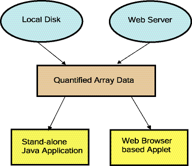
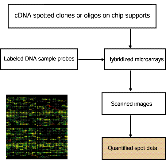
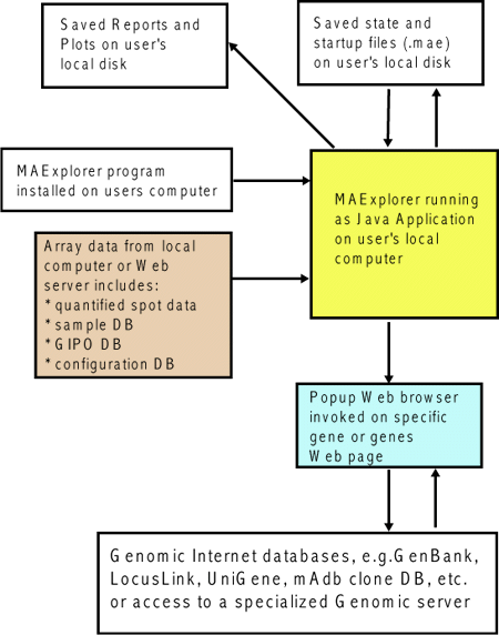
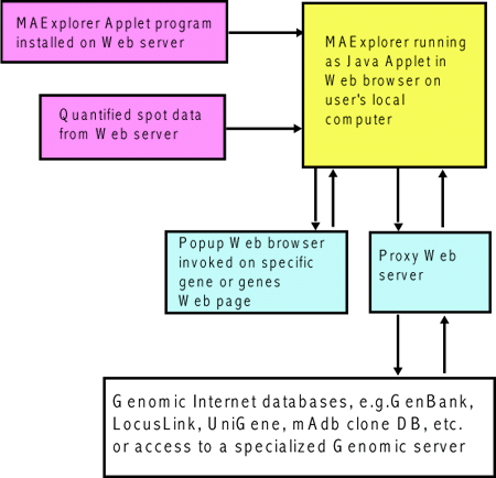


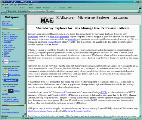
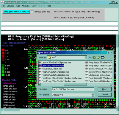

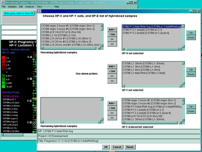
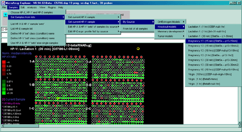
![Switching current X or Y sample by clicking on desired sample
in list at left edge of pseudoarray image. Switch between
X and Y by toggling '[X]' and '[Y]' of the Current Sample box.](GifsDocH/fig-HybProbeSetFromImageSmall.gif)
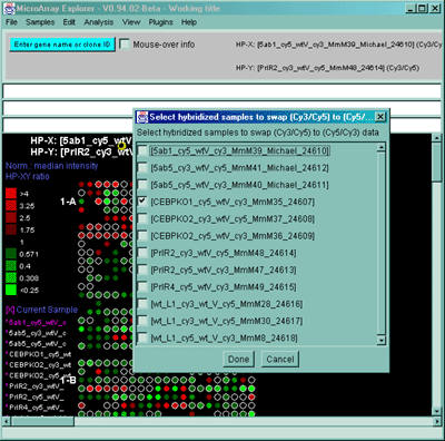
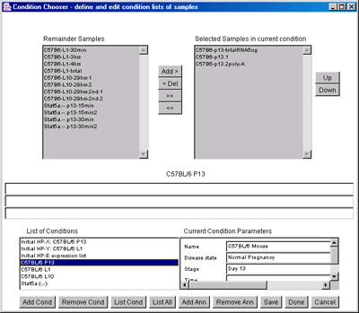
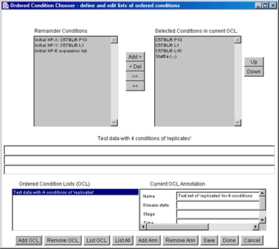
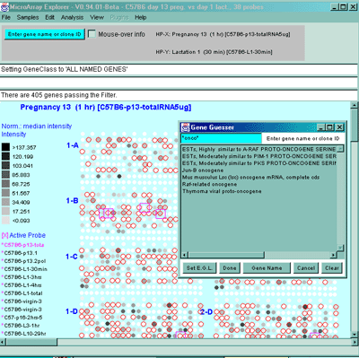


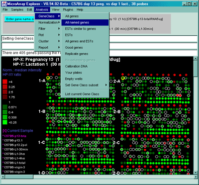
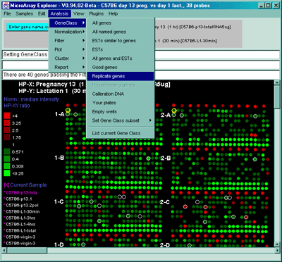
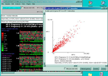
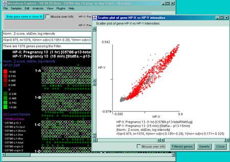
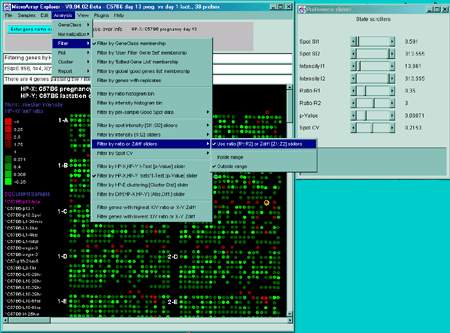


 4.1 Known Bugs in MAExplorer
