1. Introduction

This hyperlinked manual provides a detailed description of the MAExplorer conventions (Section 1) and operation (
Section 2). The latter contains many figures of computer screens showing the operations described in the Section. Section 3 discusses typical scenarios in using MAExplorer for data-mining microarrays and contains a brief introduction to the process of data mining. Section 4 lists currently known bugs and the revision history. Appendix A is a short tutorial. Appendix B is a more advanced tutorial. Appendix C describes the files required by MAExplorer and how they may be created for using MAExplorer with other array data. It also describes the data conversion tool Cvt2Mae. The Appendix D covers downloading, installing and running MAExplorer as a stand-alone Java application on a local computer. Appendix E discusses design issues for the MAExplorer Java program and supporting Web servers. Users may create new analytic methods and add them as MAExplorer Plugins as Java extensions. There is a glossary of terms used in MAExplorer. There is also a List of Figures, a List of Tables, and an Index to help find material of interest.

MAExplorer is normally used as stand-alone program

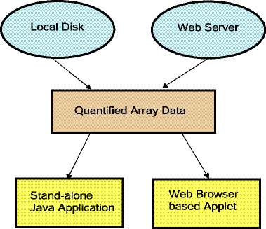
Figure 1 gives an overview of the system. Note that MAExplorer does not perform spot quantification from raw scanned images - it is used for the subsequent data mining analysis of quantified spot data. Figures 1.1.1 through 1.1.3 describe this in more detail.

Overview of MAExplorer showing it use as either a stand-alone application of Web applet

Figure 1. Overview of MAExplorer exploratory data analysis system. Initial data preparation steps are performed prior to analysis by MAExplorer and are indicated by cyan italics at the top of the figure. The primary data consists of quantified microarray image data as well as corresponding qualitative clone ID, gene-in-plate-order (GIPO or print-table, etc.), gene name, hypertext base references and related information. After the microarrays are hybridized, they are scanned and spots quantified using image spot quantification programs. These lists are then saved for each array in a tab-delimited file. Microarray image quantification may be performed by various software such as Axon's GenePix(TM), Scanalyze, Molecular Dynamics ImageQuant(TM), Research Genetics' Pathways(TM), etc. When used as a stand-alone application, data may be saved on the local computer for local off-line use, and direct access to other Internet genomic databases may be made without using a proxy server.

[DEPRICATED: When used as an applet, this auxiliary databases and the MAExplorer Jar files are copied to the Web server or local file system (in the case of the stand-alone version) where they are then available to be downloaded by users. When a user invokes a Web page containing the Java applet, it first downloads the applet that then downloads auxiliary databases including a configuration file that describes the array data. It then downloads the subset of quantified microarray spot data files requested for the set of hybridized samples being investigated. Additional samples may be downloaded at any time. When the user selects an operation that requires access to Web databases not residing on the MAExplorer Web server, implicit Java security restrictions prevent the applet from going directly to these other Web servers. Instead, it requests the MAExplorer proxy server request the data from the foreign Web server, and then returns it back to the user's Web browser. ]


Overview of MAExplorer exploratory data analysis system

Figure 1.1.1 Overview of MAExplorer exploratory data analysis system. MAExplorer is used as a stand-alone application on local data. [Its use as a Web browser applet has been DEPRICATED. In the case of the applet, it may only access quantified array data from the Web server that launched the applet.]


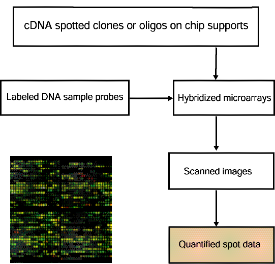
Overview of data preparation for quantified spot data used by MAExplorer

Figure 1.1.2 Overview of data preparation for quantified spot data used by MAExplorer. MAExplorer handles quantified spot data as shown in this figure. Arrays are hybridized against labeled samples are scanned and spots are quantified into spot data files. Quantified spot data is represented as tab-delimited data with data for one spot/row. Each spot is identified in this file by its grid coordinates (grid, grid row, grid column) with image (X,Y) coordinates being optional. Quantified spot data includes the raw spot intensity for each channel (in the case of multiple channels such as Cy3, Cy5, etc.). If the original data has background spot intensity values, then that may be included as well - otherwise no background data will be available for background correction. The spot data is discussed in more detail in Section 1.1 and Appendix C.1, and Appendix C.3.


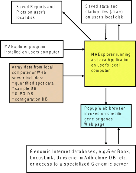
Overview of running MAExplorer as a stand-alone application

Figure 1.1.3 Overview of running MAExplorer as a stand-alone application. The preferred way of running MAExplorer is as a stand-alone application. There are distinct advantages in running MAExplorer as an application in that data and the exploration state may be saved on the users local computer, direct access to genomic servers is easier (no proxy server required - see Figure 1.4). MAExplorer plugin extensions (MAEPlugins) may only be used with the stand-alone version. Since MAExplorer is packaged for download for a variety of operating systems, using this method is not difficult to set up and the MAEPlugins should run on a variety of operating systems.


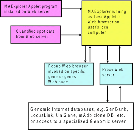
Overview of running MAExplorer as a Web browser applet

Figure 1.1.4 [DEPRICATED] Overview of running MAExplorer as a Web browser applet. An alternative way of running MAExplorer on existing databases is as a Web-browser applet. There advantage of this method is that no software installation is required on the user's computer. However, the user may not save data and the exploration state on their local computer. Furthermore, direct access to genomic servers requires a proxy server. MAExplorer plugin extensions (MAEPlugins) may not be used with the the applet version. The Mammary Genome Anatomy Program (MGAP) originally used the MAExplorer applet.


Example of a MAExplorer database - http://www.lecb.ncifcrf.gov/mae - the public MGAP DB

The Mammary Genome Anatomy Program (MGAP) microarrays of cDNA clones from mouse mammary tissue (collaboration with Research Genetics) were hybridized with 33P radio-labeled samples. These were then used to charge fluorescing plates. See the MGAP site for more documentation on the database and preparation procedures. The hybridized arrays are scanned on a phospho-imager scanner at high resolution. Spot data was quantified from these images using the Research Genetics' "Pathways 2.01" program which generated tab-delimited data files. This data also includes the microarray grid point locations (field, grid, grid row, grid col) from the associated microarray description data files (grid-in-plate-order data). When you download MAExplorer, you will also download the public MGAP dataset.

1.1 Microarrays and notation used with MAExplorer

In general, microarrays are hybridized using cDNA samples derived from mRNA labeled with either radio-label, biotin, fluorescent dyes, or other methods (see Schulze, 2001) for review of the technology). MAExplorer may be used to construct databases using single-labeled sample intensity (e.g., Affymetrix, 33P radio-labeled, etc.) and double-labeled ratio fluorescent (i.e. Cy3/Cy5) data arrays with different GIPO geometries.

Definition of "Condition list of samples"

Samples are organized into Condition Lists of samples (generally replicate samples). These may be used in various statistical and clustering tests. There are three built-in lists of samples called the HP-X 'set', the HP-Y 'set' and the HP-E list. The X and Y sets are used in various 2 condition tests such as the t-Test between the X and Y sets (Section 2.4.3). The HP-E list is an ordered expression list of samples used in clustering and in displaying expression profiles. You may interactively define new or edit named condition lists using a graphical wizard (Section 2.6), manipulate and assign them to the HP-X 'set', HP-Y 'set' and HP-E list. Some examples of condition lists might be (assuming you have the data available in your database):
  Virgin     = ( V.1, V.2, V.3 )
  Pregnacy   = ( P13.1, P13.2, P13.3 )
  Lactation  = ( L3.1, L3.2, L3.3 )
  Involution = ( I4.1, I4.2, I4.3 )

Definition of "Ordered Condition list" of multiple condition lists

We further extend this paradigm by defining a meta-data structure called the "Ordered Condition List" or OCL. This is an list of multiple conditions that you have previously defined. The OCL may be sorted if you want and the data lends itself to sorting. E.g., a time series of conditions lends itself to sorting - different types of diagnoses may not. The OCL may be used in various statistical tests (e.g., the F-test applied to the current OCL - see Section 2.4.3)). You may interactively define new or edit named Ordered Condition Lists using a graphical wizard (Section 2.7).An example of an ordered condition list might be:
  Partuition= ( Virgin, Pregnacy, Lactation, Involution )

Definition of "intensity" for single-labeled samples

MAExplorer uses the term "intensity" in slightly different ways dependent on whether you are using the single-labeled or fluorescent double-labeled data. For single-labeled data, "intensity" is the raw quantified data value as measured by the image scanner. Raw data must be normalized between samples in order to compare it between samples. Therefore, to compare N samples, you must first normalize the data and then compare them.

Definition of "intensity" for fluorescent double-labeled samples

For fluorescent double-labeled data, the Cy3 and Cy5 dye-labeled (for example) measurements are the raw quantified data values as measured by the image scanner. In this case, "intensity" is defined as the ratio of Cy3 to Cy5 (i.e. Cy3/Cy5). If you wish to look at the ratio as Cy5/Cy3, you may flip the two channels on a per-sample basis (see Section 2.2.2 for more details).

Issues of experimental design of microarray experiments

Some of the issues involved in experimental design (setting up experiments) based on the types of arrays are discussed in Section 3.1.1 for (Cy3/Cy5)-labeled as well as 33P-labeled samples. Poorly designed experiments will not yield significant statistical results, so attention should be paid to developing an adequate and robust design for your data given costs of doing experiments as well as statistical constraints on analyzing the data.

Actual and "Pseudoarray" image geometry

The main MAExplorer windows contains a pseudoarray image for visualization purposes. It may or may not correspond the spot positions on the actual array. This array geometry is defined by the number of replicate Fields (normally 1) each of which contains a number of grids (also called "blocks") containing a number of rows/grid and columns/grid of spots. If there is no explicit array geometry or spot (X,Y) coordinate data available but simply gene identifiers and intensity data, then an arbitrary pseudoarray geometry is generated. If there is an explicit array geometry, then it waill draw the pseudoarray using this geometry. The database configuration determines which method will be used and is discussed in Appendix C.5. If there is no explicit grid geometry, the number of spot Locations (e.g., IncyteID, Affymetrix probe_set) may be used to synthesize a set of grids of a size that is reasonable for viewing with MAExplorer. This is done in the Cvt2Mae array data conversion program when the array geometry (#grids, #rows/grid, #columns/grid) is not known. This conversion is not done in MAExplorer itself. In Cvt2Mae we generate a visually appealing pseudoarray image geometry if no array geometry is specified with the data (e.g. Affymetrix data, etc). It maps the number of N spot data entries to a (#grids,#grid-rows,#grid-columns). The algorithm is given in Appendix C.6 as well as a suggestion for handling non-standard geometries using Cvt2Mae.

Gene coordinate numbering on the microarray

A
gene coordinate numbering is a mapping of gene identifiers to locations on the array for a particular array geometry. These are described by grids (or blocks), each consisting of grid rows by grid columns of spots. The grids may be repeated on the array and constitute duplicate fields. Some arrays group subsets of grids into meta-grids which are specified by meta-grid rows by meta-grid columns of grids. MAExplorer can handle grids but not meta-grids. In the case where there is no array grid geometry specified or meta-grids are used, an arbitrary pseudoarray geometry can be constructed to serve as a basis to display the microarray pseudoimage (see the Algorithm for constructing the pseudo array from a list of spots in Appendix C.6).

In MAExplorer we refer to grids by letter names (A,B,C,...) and fields by F1 and F2. If you are using Cy3/Cy5 ratio data and the Cy3 and Cy5 data is available as independent channels for each HP sample, then operations that use F1 and F2 will use the Cy3 and Cy5 data for various operations such as scatter plots (Cy3 vs Cy5), etc. If there is only one field in an array (i.e. no duplicate grids), then when MAExplorer is run, operations and menus describing F1 and F2 operations will not be available.

Using duplicate (F1 and F2) spots allows us to get an estimate of the hybridization variance within an array and is used to compute the (F1,F2) gene coefficient of variation (CV) used in the gene data Filter to remove noisy data before looking for additional differences. Note that if Cy3/Cy5 data is used, then F1 and F2 duplicates are not allowed as MAExplorer uses the (F1,F2) data to hold the(Cy3,Cy5) data for a hybridized sample.
Example: special array spot coordinate numbering for the MGAP array

As an example of this coordinate system, the following describes the array geometry for the array used in the NIDDK MGAP database. The general principal with different sizes and numbers of fields is the same for other arrays. The MGAP array was spotted by Research Genetics for MGAP. Clones in the array are laid down in grids consists of 8 rows and 24 columns per grid. There are 8 grids (named A through H or 1 to 8) to a field with a space between grids. Finally, there are two fields (left and right named 1 and 2 or F1 and F2) that are duplicates.

Note: we currently present the MGAP arrays with grids A through H oriented from top to bottom - whereas Research Genetics orients them rotated +90 degrees with grid H to the left and grid A to the right. This occurred when the images were scanned with a -90 degree change in the orientation. Therefore, we have swapped rows and columns in our relative orientations so it meets with users normal expectations of row-column orientation. This could be easily changed to the Research Genetics convention using a parameter in the configuration file. Since the actual plate coordinates are tracked with each clone and reported when it is accessed in MAExplorer, the image coordinate system is not that critical - although the verisimilitude of actual array layout and the data-mining layout can be useful.

Setting the "current gene" to a specific gene by "Master gene ID"

The MAExplorer uses the concept of the "current gene" to indicate a particular gene to be analyzed. You may interrogate the microarray database or Internet databases for data on the current gene or to use it in one of the operations. For example, you might cluster genes by expression profiles to find other genes with profiles similar to the current gene.

Various gene identifiers may be present in the GIPO data file associated with the array. One of these is selected to as a unique identifier to represent genes in the MAExplorer database. Normally, the Master gene ID is defined as the Clone ID. However if the Clone ID is not present, but the GenBank ID is, it will use the latter as the identifier. If neither GenBank nor Clone ID is present, it will use GenBank5' then GenBank3' if present. If that is not present, it will use the UniGene ID if is present. If that is not present, it will use dbEST5' then dbEST3' if present. If that is not present, it will use LocusLink LocusID if present. Finally, if none of those identifiers are present, you can specify a 'Generic ID' that is related to some other database gene identifier such as a 'Location' identifier.

The current gene may be specified by clicking on a spot in the microarray image or on a point in the popup scatter plot, or a gene ID cell in a report.

Setting the "current gene" by Gene Name Guesser

In addition, the user may type a specific gene name or clone ID into a popup Gene Name Guesser dialog text window. This is invoked by clicking on the blue button "Enter gene name or clone ID" at the top right in the control panel. When the "guesser" window pops up, start typing the gene name or clone ID in the blue text entry field. You select either the Gene Names, Clone ID, UniGene ID, GenBank, GenBank 3' or GenBank 5',dbEST 3', dbEST 5', or LocusID identifier. Then you may start typing letters and it will match all names or identifiers which are prefixed with the sub-string you have typed so far. As you type more characters, it will limit the list of possible completions of what you are typing. After selecting the gene you want, you then press the "Done" button to use this entry to set the current gene and remove the guesser popup window. You may press the "Clear" button to clear what you have typed and the "Cancel" button to cancel the current gene selection process.

Setting the "Edited Gene List" subset of genes using wildcard names

You may also define a set of genes from the guesser window using wildcard names where the character '*' matches zero or more characters. First you specify a sub-string common to gene names. Then press the "Set E.G.L." (set 'Edited Gene List') button. For  
example (see Figure 2.3.1), you could find all oncogenes and proto-oncogenes by typing "*ONCO*" in the guesser. It automatically enables the View 'Edited Gene List' in the array that shows genes in the E.G.L. enclosed in magenta boxes.

The current gene cluster

Some operations involving clustering will automatically assign the gene cluster to the E.G.L. This includes clustering of genes similar to a selected (i.e. current) gene and K-means clustering. In the case of K-means clustering, the cluster you select by picking a gene belonging to that cluster will cause it to be defined as the current cluster and also assigned to the E.G.L. This will be discussed in more detail in the section on clustering.

The current Condition List of samples

The current
condition list of samples is the last condition edited with the interactive graphical wizard (Section 2.6) used to define new or edit condition lists.

The current Ordered Condition List (OCL) of multiple conditions

The current ordered condition list (is a possibly ordered list of Multiple Condition Lists) is the last condition edited with the interactive graphical wizard (Section 2.7) used to define new or edit ordered condition lists.

Saving full resolution plots as GIF files in stand-alone mode

The various plots may be saved as full resolution GIF files when running MAExplorer in stand-alone mode. The various plots have "SaveAs" buttons which appear in stand-alone mode. Saving your intermediate results may be useful for documenting your data mining session or for subsequent publication. (Here is an example of a full resolution clustergram of 38 MGAP hybridized samples for 1076 named and EST genes).

Saving Text windows as .txt files in stand-alone mode

The various text windows may be saved as .txt files when running MAExpplorer in stand-alone mode. The various text windows have "SaveAs" buttons which appear in stand-alone mode. Saving your intermediate results may be useful for documenting your data mining session or for subsequent publication.

1.2 Microarray image quantification

Quantification data for all genes in a hybridized sample (x and y coordinates, intensity, background density) is obtained by reading data from a quantification file for that hybridized sample. The quantification file for each hybridized sample resides on the local file system (for stand-alone) or MAExplorer Web server (for applet use) and is derived from image quantification programs such as Axon's GenePix(TM) program, Scanalyze, Molecular Dynamics' ImageQuant(TM) program, Research Genetics' Pathways(TM) program, etc.   These programs are independent of MAExplorer and are not part of our downloadable software distribution. Normalization between hybridized samples must be performed to allow comparison between different hybridized array samples. File formats are discussed in Appendix C).

1.2.1 Ratio and Zscore comparison of data from different hybridized samples

Because of variation between hybridized samples, data is normalized. Methods that are pure scaling transformations (such as Median, Scale to 65K, By Calibration DNA, By Use Gene Set, etc.) allow you to compare data using the ratio between two normalized sets of data. We define the ratio for two samples as follows:
    ratio(x,y,c) = Ixc / Iyc
where: 
    samples x,y have values Ixc and Iyc for the same 
    gene c in samples HP-X and HP-Y
The Zscore method transforms the data such that it can not be used with the ratio comparison. Instead we use the Zdiff(x,y) method for comparing Zscore developed by Mark Vawter (Vawter, 2000). Zscores typically cover the range of -3.0 to +3.0 (standard deviations) with a transformed mean of 0.0. Therefore the Zdiff will typically cover the range of -6.0 to +6.0.
Let
    Zscore(p,c) = (Ipc - meanp)/stdDevp
where:
    Ipc is the intensity of gene c for sample p. Sample p has meanp 
    and stdDevp

Then,
    Zdiff(x,y,c) = Zscore(x,c) - Zscore(y,c),
where: 
    samples x,y have Zscore(x,c) and Zscore(y,c) normalized values for the 
    same gene c in samples HP-X and HP-Y, or HP-X 'sets' and HP-Y 'sets'.

Table 1.2.1 Displays affected by the normalization mode. When comparing two hybridized samples or sets of hybridized samples, the metric used is either ratio or Zdiff depending on whether the Zscore normalization was selected in the Normalization menu. This will affect a variety of data displays and some of the data Filter methods listed here. In addition, all of the other graphics (EP plots, intensity histogram plot, cluster plots including clustergrams and dendrograms) are also affected by the normalizations.

  1. Pseudocolor X/Y ratio, X-Y Z-diff, and other pseudoarray images
  2. the 3-line gene data displayed in the main MAExplorer window
  3. the gene data display at the top of the scatter plot when clicking on a point in the scatter plot
  4. report tables of genes with the highest/lowest X/Y (Cy3/Cy5) (F1/F2) ratio or X-Y (F1-F2) Zdiff
  5. Ratio histogram plot of X/Y (Cy3/Cy5) (F1/F2) ratios or X-Y (Cy3-Cy5) (F1-F2) Zdiff data
  6. data Filter: Spot Intensity [SI1:SI2] range or Zdiff [Z1:Z2] range for HP data
  7. data Filter: Intensity [I1:I2] range or Zdiff [Z1:Z2] range for (HP-X/HP-Y) or (HP-X - HP-Y) data
  8. data Filter: Ratio [R1:R2] range or Zdiff [Z1:Z2] range for (HP-X/HP-Y) or (HP-X - HP-Y) data
  9. data Filter: Ratio [CR1:CR2] range or Zdiff [CZ1:CZ2] range for (Cy3/Cy5) or (Cy3-Cy5) data of a single sample
  10. Range and scale of data in EP plots, cluster plots, clustergrams, dendrograms, etc.
  11. Statistical tests t-tests (X and Y sets), Kolmogorov-Smirnov test (X and Y sets), ANOVA F-test (OCL), etc.


1.3 Microarray image and plot display

The MAExplorer displays one microarray pseudoarray image of the hybridized samples. This is either for a single sample, the ratio of two samples, the average of replicate samples or the ratio of two sets of replicate samples, the ratio Cy3/Cy5 or Cy5/Cy3, or other mappings. Section 2.4.4.1 Show microarray pseudoarray images menu describes these options and shows some examples.

The Filter menu is used to select a set of data filters that determines which genes are selected. These are highlighted in the array image in different ways - with a red (white) circle in the intensity (ratio) pseudoarray image each spot meeting the range threshold criteria. How these are highlighted depends on which Plot menu Show Microarray method and View menu modes were selected. If the Show 'Edited Gene List' (EGL) option is set in the View menu, genes in the EGL will appear as magenta squares. The "Filter mode" is always present and shows genes meeting various Filter criteria (to be discussed). The user may interactively define a list of genes by clicking on them when the Click to add gene to edited gene list option is set in the Edit menu. Alternatively, you can click on a gene with the Control key pressed to add a gene to the EGL or with the Shift key pressed to delete a gene from the EGL.

Types of pseudoarray image displays

There are several differnt types of pseudoarray images that may be displayed. The current type is set in the Show Microarray submenu in the Plot menu selections including Pseudograyscale intensity that approximates the intensity of a single sample or average of samples. The Pseudocolor Red(X)-Yellow-Green(Y) HP-X/HP-Y ratio or Zdiff and Pseudocolor Red(Cy5)-Yellow-Green(Cy3) Cy3/Cy5 (or F1/F2) ratio or Zdiff add the two samples or channels together as separate Red+Green channels to give a color spectrum. The Pseudocolor HP-X/HP-Y ratio or Zdiff Pseudocolor Cy3/Cy5 (or F1/F2) ratio or Zdiff gives a color spectrum from a low ratio (zdiff) value (Green) to a high value (Red) with a value of 1.0 (0.0) of Black. The Pseudocolor (HP-X,HP-Y) 'sets' p-value shows the p-Value between two X and Y sets in a color spectrum.. If the Original image is set and the image file is in the database, it will pop up a separate Web browser window to display it. The Pseudograyscale display is a grayscale image, with higher concentration genes appearing darker, on a light blue background. The pseudocolor HP-X/HP-Y ratio of spots image is constructed using a color scale going from bright green (<1) to black (=0) to bright red (>1) on a black background. For the pseudocolor Zdiff of (X-Y), the color scale goes from bright green (<0) to black (=0) to bright red (>0). If the dichromasy switch is set in the View menu, that a different set of colors is selected that may be easier for some people to differentiate. If the Use dual HP-X & HP-Y 'sets' else single samples toggle in the Samples menu is set, it displays the mean HP-X data in the left and HP-Y in the right for doing a side by side comparison.

In all of the pseudoarray images, the grids in the image are labeled field#-GridLetter (e.g. 1-C, 2-B, etc). This allows them to be clearly identified as the user scrolls over the image that is larger than the visible computer window.

Popup windows

MAExplorer starts with the main pseudoarray image windows. This window contains the pull-down menus where you may issue commands. As you perform various operations, new windows may popup for some of these commands. For most of these windows, you may click on the "Close" button or click on the close window icon associated with your operating system (generally one of the buttons at the top of the popup window). However, some windows were designed to not close when you do this. In particular the "State sliders" are not able to be closed unless the associated data filtering or clustering operation is closed. When you close the associated operation will automatically close the state slider window.

There is also a popup alert message window for bettering informing users of conditions that prevent them from doing the operation they requrested. You must press the Close button to pop-down the message, although you may do press the SaveAs butto to save the message to a file. For complex problems, some of the messages may suggest what you need to do to correct the problem.

The current sample sample, HP-X, and HP-Y

In MAExplorer, a hybridized array sample is abbreviated HP. The underlying data comparison model assumes, as a minimum, the comparison of two different experimental conditions represented by samples HP-X and HP-Y. A good way to think about this is that these variables are the two axes of a scatter plot (one of the displays you may generate). The HP-X and HP-Y may be thought of as containing data from either single hybridized samples or containing mean data from multiple replicate sets of sample. The HP-X and HP-Y are assigned using the Set current HP-X and Set current HP-Y in the Samples menu (hybridized sample is abbreviated HP in MAExplorer. The sets are most easily changed using Choose HP-X, HP-Y and HP-E to select the currently active samples. The contents of the of multiple sample HP-X and HP-Y 'sets' may alternatively be changed using the Edit HP-X & HP-Y 'sets' of samples by source submenu, and the HP-E list of samples using the Edit HP-E list of samples by source. Assigning single samples to either HP-X or HP-Y may be done from the Samples menu. However, it is easier to do it by clicking on the pseudoarray image. First click on the magenta "[X]" or "[Y]" Current Sample box at the top of the list of switch between HP-Y and HP-Y. Whichever is visible ([X] or [Y]) is the one that will be the HP sample assigned. Then simply click on the magenta "*" to the left of the sample name for the sample you wish to assign.

Hybridized samples are selected from a list of all of the sample samples in the database. To make it easier to select a HP, they may be selected from submenus by their developmental stage (if supported by your particular database) or from a list of all samples in the database located on the left side of the pseudoarray image. If a sample has never been loaded during a session, it will be loaded when you request it.

The last sample selected is called the current sample or current HP. That is the sample that is displayed in the pseudoarray image in the primary MAExplorer window when using display modes requiring a single sample.

Using 'sets' of HP-X and sets of HP-Y

Multiple samples may be assigned to the to the HP-X or HP-Y sets. These are assigned using the Edit HP-X and HP-Y 'sets' of microarrys in the Samples menu. The multiple sets are enabled by setting the Use HP-X and HP-Y 'sets' else single samples checkbox in the Samples menu. Then, when statistical calculations are performed on that data, it will use the means, std-deviations, etc. from each of these sets rather than individual samples.

The HP-E sample list for computing expression profiles

You may cluster sets of genes with similar expression profiles across a set of hybridized samples. The set of HP samples used in doing these profiles is specified by Edit expression profile 'list (HP-E) in the Samples menu. The Choose HP-X, HP-Y, and HP-E command may also be used for defining the members and order of the samples in the HP-E 'list'. Then, gene intensity expression profiles may be created in a popup window for hybridized samples in the HP-E set by using the Expression profile plot commands in the Plot menu. Several of these plots may be created on the screen at the same time. Clicking on a vertical data line in the plot will show the name of the HP, its intensity and coefficient of variation (CV) of the (F1,F2) data for this gene. Note that you can order the hybridized samples in the HP-E set by the order in which they are added.

Data 'Filters' - the intersection of one or more data tests

A set of genes may be computed by taking the intersection selected gene sets. These sets are determined by various logical, data range and statistical tests. Genes passing each test are assigned to a gene subset which in turn are used in the gene intersection computation. The final gene subset is used in array, plots, and reports, and subsequent data filtering. Changing any test parameters causes the data filter to be re-computed.

List of data filters for MAExplorer - any number of filters may be used simultaneously

Figure 1.3 Data Filter Venn diagram. This illustrates some of the logical, data range and statistical tests criteria available using the MAExplorer data Filter paradigm. Note that multiple criteria may be selected from each of these categories. The extreme case, probably never used, could use all tests.


1.4 Exploratory data analysis - overview

MAExplorer may be used to perform various data explorations by looking for patterns correlated with different sets of hybridized samples or with expression profiles of genes. This is discussed in more detail throughout this manual and later in Section 3 on Exploratory Data Analysis. Detailed descriptions of all commands are given in Section 2 Menus.

A first-approximation approach to data-mining might be to sequentially constrain the data of interest to find some changes and then to report on those changes. We have arranged these commonly performed first-pass operations as submenu entries in the Analysis Menu. The submenus are:

  1. GeneClass Menu
  2. Normalization Menu
  3. Filter Menu
  4. Plot Menu
  5. Cluster Menu
  6. Report Menu

The primary 'Analysis' menu of MAExplorer - most operations are found in this menu

Figure 1.4 Screen view of MAExplorer main window with Analysis Menu. The menu structure of MAExplorer was designed to allow users to quickly perform commonly used data-mining operations. Other menus are used for modifying the data (File, Samples, Edit, and View menus) or accessing on-line Help menu information in a separate Web browser popup window. MAExplorer menus are similar to most Windows PC applications where pull-down menu selections are used to invoke operations. The current hybridized array sample is displayed as a pseudocolor ratio image of median normalized spot intensities. Clicking on a spot assigns it as the current gene with data being reported in the top most message area. The names of the current HP-X and HP-Y samples are listed above that area. In general, clicking on spots, points in plots or cells in spreadsheet reports will assign the it as the current gene and access Web genomic databases if enabled.


In addition to displaying the hybridized sample pseudoarray images, derived data may be viewed in various types of plots. These include scatter plots, histograms, ratio-histograms, expression profiles, gene clustering, etc. Data may be presented as table reports presented as either active spreadsheets that can access genomic databases by clicking on cells or as tab-delimited Excel-compatible tables that may be cut (if your windowing system supports this) and pasted into an Excel spreadsheet.

The selected HP-X and HP-Y samples are used when generating scatter plots, ratio histograms and other graphics. Scatter plots and ratio histograms may also be performed on the left and right sides of the currently displayed HP array (fields F1 and F2 respectively if array data has duplicate spots for the same genes).

A MAExplorer database contains a table identifying genes, so data is accessible by gene name as well or by sub-strings identifying a set of genes (e.g. "onco" that could be used to find any oncogene or proto-onco gene in the database).

When the program starts, it displays the microarray image of the first hybridized sample in the HP-X set of samples initially specified. If you specify a new HP-X or HP-Y sample, then it changes the pseudoarray image to correspond to that array. You may change the current HP-X or HP-Y sample from either the Samples pull-down menu or by clicking on a sample in the Active Sample list in the left of the pseudoarray image. If you click the mouse on or near a spot, it will latch onto that spot and define it as the current gene.

Note: In Figure 1.4, genes that pass the MAExplorer data Filters are indicated by red (white) circles around spots in the pseudograyscale (pseudocolor) intensity (ratio) image. The pseudoarray image shows the gene data as replicate grids of spots if there are two fields Field 1 (left set of grided spots) and Field 2 (right set of grided spots). If there is no duplicate spot data, then only Field 1 is shown.

If background correction is enabled in the Normalization menu, then intensity is reported in the message displays as intensity' otherwise as intensity. Normalization should also be used between hybridized samples - whether the data is ratio data (i.e. Cy3/Cy5) or single sample intensity arrays.

1.4.1 Saving the state of a data-mining session in stand-alone mode

If you are running MAExplorer in stand-alone mode, you may save the state of your session for later use using the "Save DB" or "SaveAs DB" commands. Then, the checkpointed database could be accessed using the "Open file DB command". It currently saves: the gene sets, condition (HP) lists, current HP-X, HP-Y and HP-E lists, data Filter options and slider value settings, display options, clustering options, normalization options, etc. We recommend using the "SaveAs ... DB" so you can save the state under a different name rather than overriding the original state. This way you could backup to the original state if you wanted to. The "SaveAs DB" and "Open file DB" commands are described in the File menu.

1.4.2 Logging messages and command history

Often a user would like to review measurements of particular genes and to review the list of commands they issued (also called the command history). Various data measurements as well as many other types of information in the three text lines in the status area of the main window may optionally be recorded in a
popup message log (Section 2.5.1) and the command history may also be reviewed in a separate popup message log (Section 2.5.2). If you are running the stand-alone version, the logs may be saved. Otherwise, you could cut and paste the log data into other word processing applications.

1.5 Quick start - demonstration of MAExplorer

MAExplorer is used as a stand-alone application. You may
download the stand-alone application (see Appendix D). This download also include a demo data set of 50 hybridized samples from the public MGAP database. In any case, you can explicitly download the data at any time at http://www.lecb.ncifcrf.gov/mae/MGAP-Array-database.zip or HREF="http://prdownloads.sourceforge.net/maexplorer/MGAP-Array-database.tar.gz?download"> http://prdownloads.sourceforge.net/maexplorer/MGAP-Array-database.tar.gz?download

Setting up MAExplorer to work with user-specific data is discussed later in this manual in Appendix C.

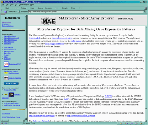
MAExplorer Home page

Figure 1.5.1 The MicroArray Explorer home page at http://maexplorer.sourceforge.net/. The table of contents in the left panel lists an introduction and short tutorial, several demonstration databases. Below that are links to documentation including this reference manual, glossary and index. The Export version discusses running MAExplorer with other arrays and as a stand-alone version. The Download application is a Web page for downloading and installing the stand-alone Java application on your computer.


You may start MAExplorer in your Web browser from the MGAP Startup DB. This offers several preset public databases consisting of sets of hybridized samples as well as the empty database. After you have clicked on a particular startup database, it will begin loading MAExplorer - indicated by a red box with a "Loading..." message in the top window of your browser. After MAExplorer starts, this message changes to a white box with "Reading DB" while it downloads the data files required. Finally, when it is ready for your interaction, it displays a white box with a green "Ready".

NOTE: for Web browser invocation, the MAExplorer applet works with Netscape 4.7, Internet Explorer 5.0, and HotJava on a Windows (95/98/NT/2000/XP) system or a Solaris Unix system. Macintosh and SGI systems seem to hang at times because of Web browser problems. However, it works on all other systems as a stand-alone Java application that you may download and install on your computer. You might want to review these Web browser restrictions.

After the MAExplorer is started and the menus become active, you may switch the preset hybridized samples to other samples using the Samples pull-down menu. The last hybridized sample loaded becomes the "current hybridized sample" and its image is the one displayed.

Exiting MAExplorer

If you are in MAExplorer and want close the program and exit, you may use the Quit command in the File menu or click on the "close application" button (found in the upper right hand corners of MAExplorer windows put there by your operating system).

1.6 Tutorials for using MAExplorer

There are a number of things you may do in this data mining facility.
  1. Analyze expression of individual genes
  2. Analyze expression of gene families and clusters
  3. Compare expression patterns in multiple hybridizations
We wrote two tutorials to help you understand its capabilities. We recommend you first try the
short tutorial before attempting the advanced tutorial. The latter demonstrates some of the more advanced capabilities.